• Morphology Reconstruction & Visualization
  • What is a Morphology Skeletion?
  • Morphology Components
  • Why this Toolbox?
    • Morphology Analysis Tools
    • Morphology Visualization Tools
  • User Interface
  • Opening the Morphology Reconstruction Toolbox
• Morphology Reconstruction Method
  • Disconnected Sections
  • Disconnected Segments
  • Connected Sections
  • Articulated Sections
  • Progressive
  • Samples
  • Dendrogram
• Morphology Reconstruction Parameters
  • Skeleton Style
    • Original
    • Tapered
    • Zigzag
    • Tapered Zigzag
    • Straight
  • Branching Method
    • Angles
    • Radii
  • Arbors to Soma
    • Connect Connected
    • All Connected
    • All Disconnected
  • Resampling
    • None
    • Adaptive Relaxed
    • Adaptive Packed
    • Fixed Step
  • Arbor Quality
  • Radii
    • Original
    • Unified
    • Type Unified
    • Scaled
  • Soma
    • Ignore
    • Sphere
    • MetaBalls
    • SoftBody
  • Maximum Branching Order (per type)
• Colors and Materials Options
• Morphology Rendering: Let's Render a Morphology
  • Wide Shot
  • Mid Shot
  • Close Up
  • Rendering Resolution
    • Fixed
    • To Scale
  • Camera View
  • Rendering Animation
    • 360
    • Progressive
  • Morphology Export Options
    • SWC
    • Segments
    • Blender
• Navigation

This panel gives access to the parameters of the Morphology Reconstruction Toolbox. By reconstruction in the context, we mean drawing a three-dimensional skeleton from a morphology file that was originally reconstructed from an optical microscopy stack.

Neuronal morphologies are reconstructed from imaging stacks obtained from different microscopes. These morphologies can be digitized either with semi-automated or fully automated tracing methods. The digitization data can be stored in multiple file formats such as SWC and the Neurolucida proprietary formats. For convenience, the digitized data are loaded, converted and stored as a tree data structure (a data structure representing the dendrogram).

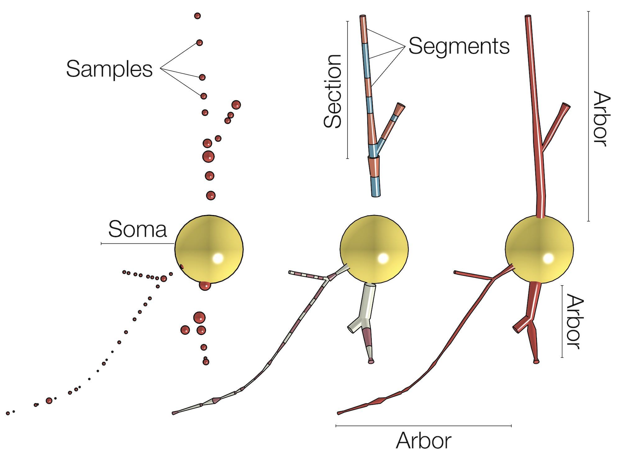
The skeletal tree of a neuron is defined by the following components: a cell body (or soma), sample points, segments, sections, and branches. The soma, which is the root of the tree, is usually described by a point, a radius and a two-dimensional contour of its projection onto a plane or a three-dimensional one extracted from a series of parallel cross sections. Each sample represents a point in the morphology having a certain position and the radius of the corresponding cross section at this point. Two consecutive samples define a connected segment, whereas a section is identified by a series of non-bifurcating segments and a branch is defined by a linear concatenation of sections.

Neuronal branches are, in general, classified based on their types into

• axons,
• apical dendrites and
• basal dendrites.

Note that the three-dimensional profile of the soma that is reconstructed in this skeleton - if requested - is based on the parameters set in the Soma Toolbox panel.

There are various packages that have been developed to analyze and visualize different formats of neuronal morphology skeletons. Free and open source packags are quite limited in their functionality and some of them require installing multiple software dependencies that might make them cumbersome and hard to use. Non-free or proprietary solutions might not be affordable in certain cases and they are only focused on morphology visualizatin. NeuroMorphoVis close the gap and presents a free framework for advanced visualiztion of the morphologies, visual analysis, mesh generation of neuronal membranes and high quality rendering for scientific publications, all integrated in a single tool.

For the record, we list other packages that are used to analyze and visualize morphology skeletons.

• MATLAB-based Morphology Analyzer by J. Ledderose et al, 2014.

• HBP Morphology Viewer by HBP - Online repository can be found here.

• NeuronLand: NLMorphologyViewer A simple user interface built on top of the technology developed for the NLMorphologyConverter. Provides a 3D interactive view of neuron morphology data.

• Web-based neuron morphology viewer by R. Bakker and P. Tiesinga, 2013.

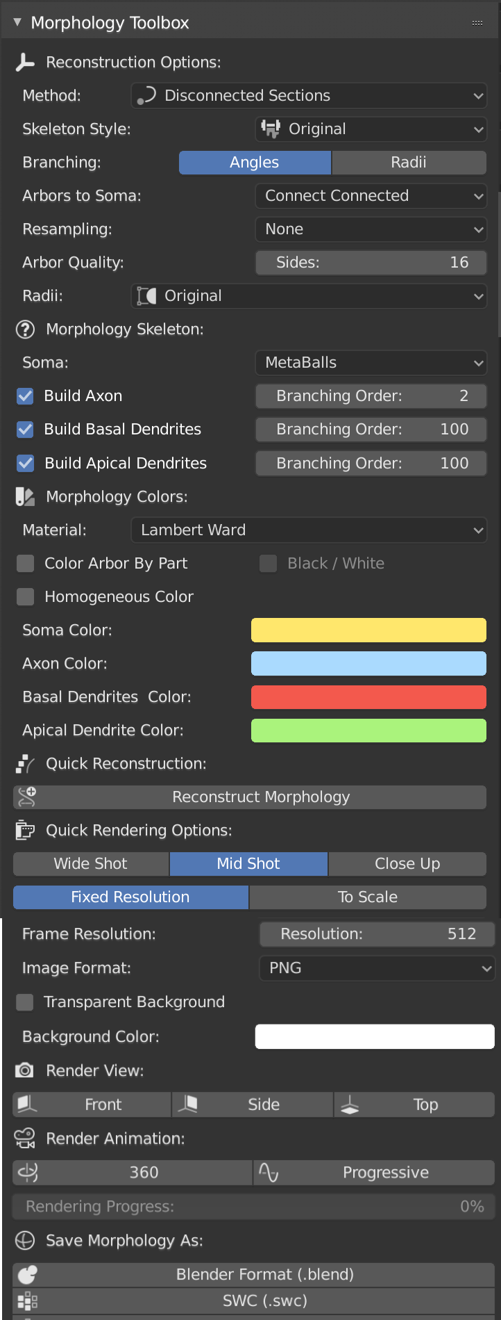
When you toggle (or click on) the Morphology Toolbox tab highlighted above, the following panel, or a similar one depending on the version of NeuroMorphoVis, will appear.

NeuroMorphoVis has support to reconstruct (or draw) neuronal morphologies using various methods including:

• Disconnected Sections
• Disconnected Segments
• Connected Sections
• Articulated Sections
• Progressive
• Samples
• Dendrogram

The method can be selected in GUI from the Method drop down list under the reconstruction options as shown below.

The morphology reconstruction method can also be set in the configuration file as follows:

## Morphology reconstruction method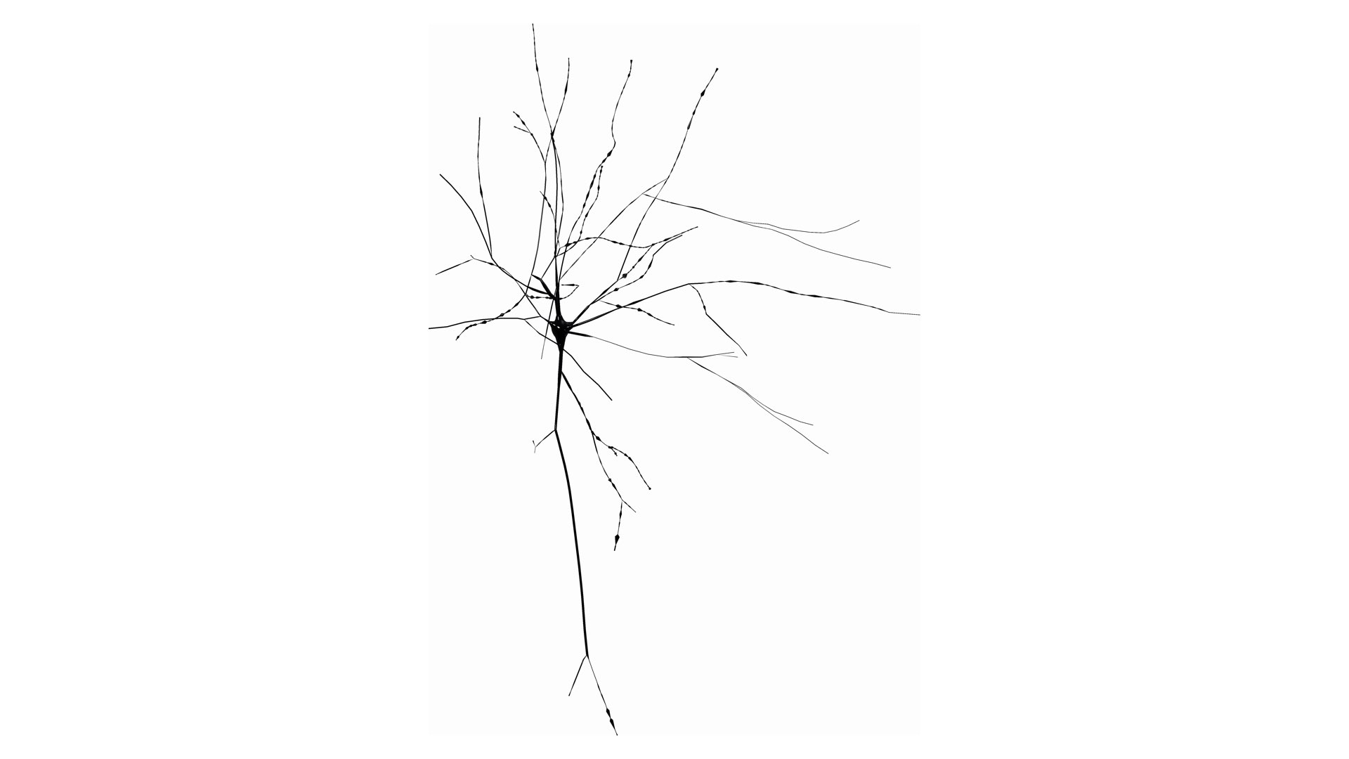   
MORPHOLOGY_RECONSTRUCTION_ALGORITHM=disconnected-sections

The morphology skeleton is drawn as a list of sections, where each section is an independent object that is disconnected from the neighboring sections. The section object is a polyline composed of a list of samples. Note how each section is assigned a different color in the following image.

This mode can be set in the configuration file as follows:

# Morphology reconstruction method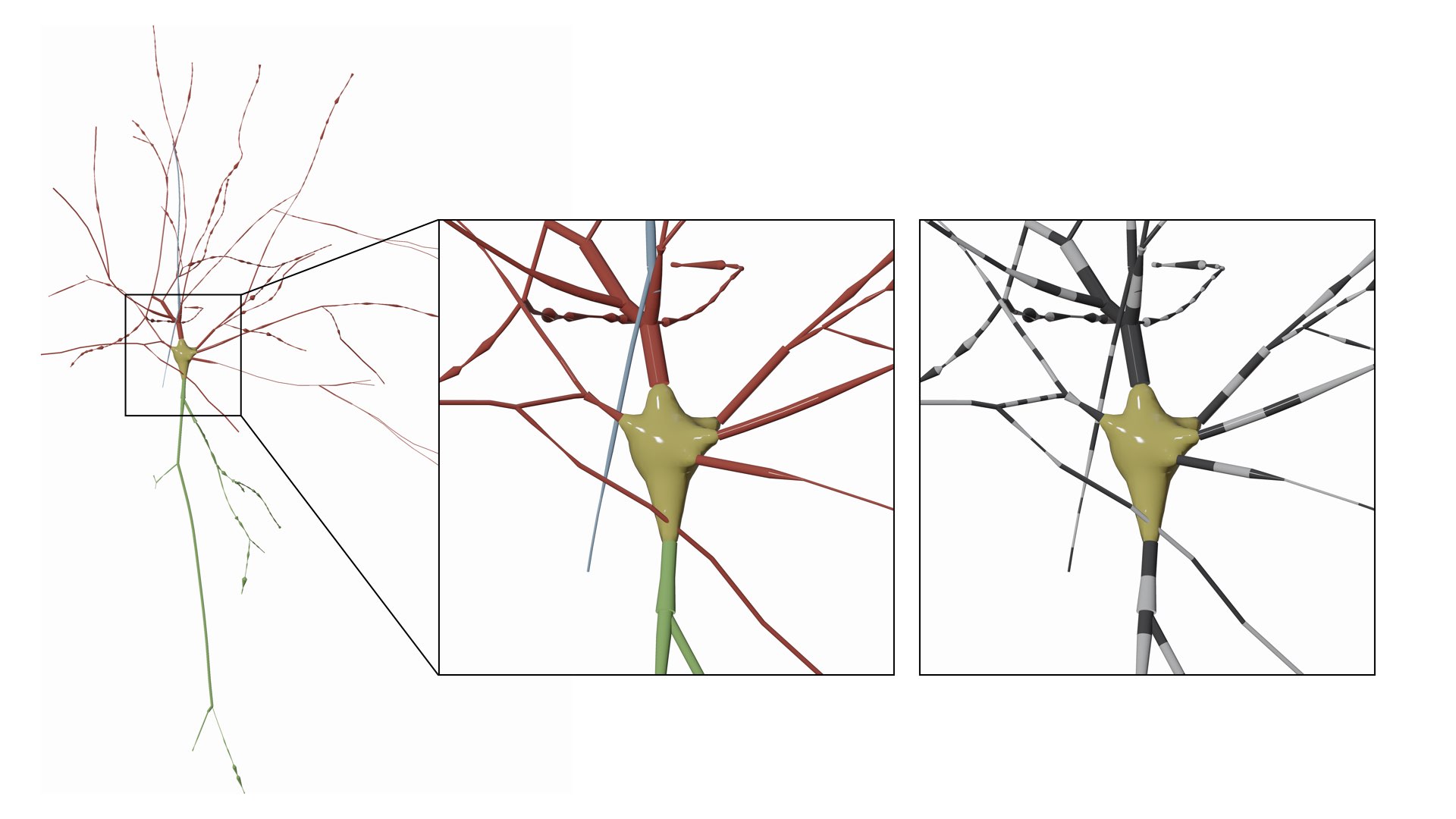
MORPHOLOGY_RECONSTRUCTION_ALGORITHM=disconnected-sections

Each segment in the morphology is drawn as an independent object that is disconnected from the neighboring segments. The segment is a simplified polyline reconstructed from connecting two samples only along the section. This drawing scheme is very useful to visualize and debug the sampling of every section. Note how the segments in the morphology are assigned alternating black and white colors in the following image.

This mode can be set in the configuration file as follows:

# Morphology reconstruction method
MORPHOLOGY_RECONSTRUCTION_ALGORITHM=disconnected-sections

This method draws the morphology as a series of connected sections like a stream from the root section to the leaf on every arbor.

This mode can be set in the configuration file as follows:

# Morphology reconstruction method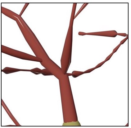
MORPHOLOGY_RECONSTRUCTION_ALGORITHM=connected-sections

This mode is similar to the Disconnected Sections method, but between every two sections a sphere is inserted as an articulation.

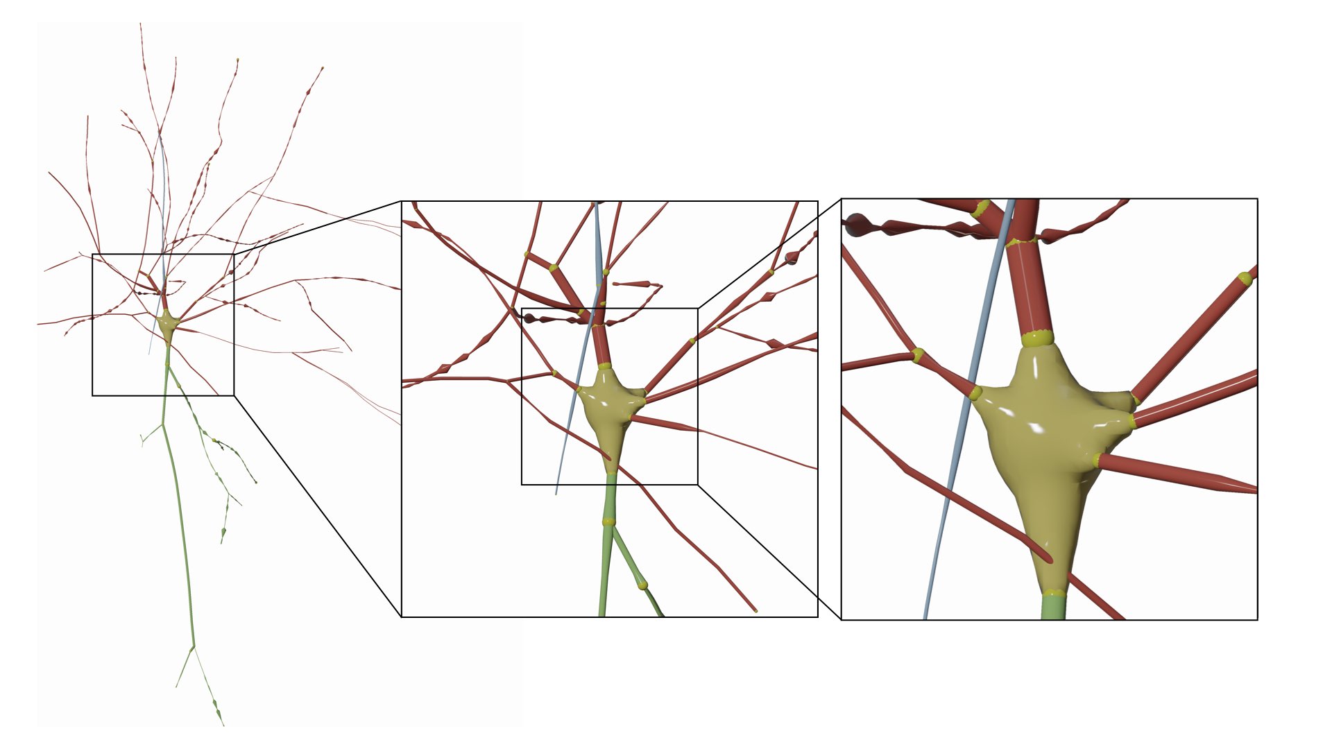
This mode can be set in the configuration file as follows:

# Morphology reconstruction method
MORPHOLOGY_RECONSTRUCTION_ALGORITHM=articulated-sections

This mode visualizes the progressive generation of the arbors from the soma.

To visualize the progressive reconstruction of the neuron, select the Progressive mode from the Methods menu, and then click on the Play button as shown below.

This mode is only allowed from the GUI. It cannot be set in the configuration file. Nevertheless, a progressive reconstruction sequence can be generated from the configuration file by setting the following rendering parameter to yes:

# Render a sequence of frames reflecting the progressive skeleton reconstruction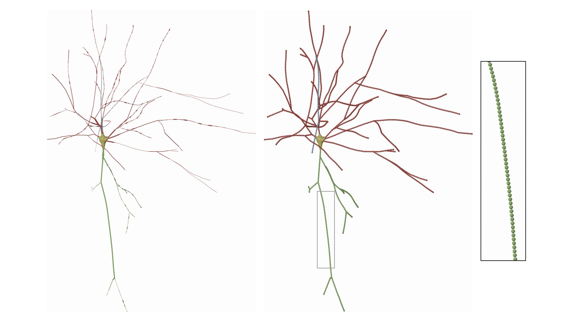 
RENDER_NEURON_MORPHOLOGY_PROGRESSIVE=yes

The morphology is drawn as a list of spheres, where every sphere represents a sample in the morphology. This mode is useful to visualize the distributions of the samples along the arbors, but it might take several seconds to draw all the spheres for a relatively large morphology (with more than 5000 samples).

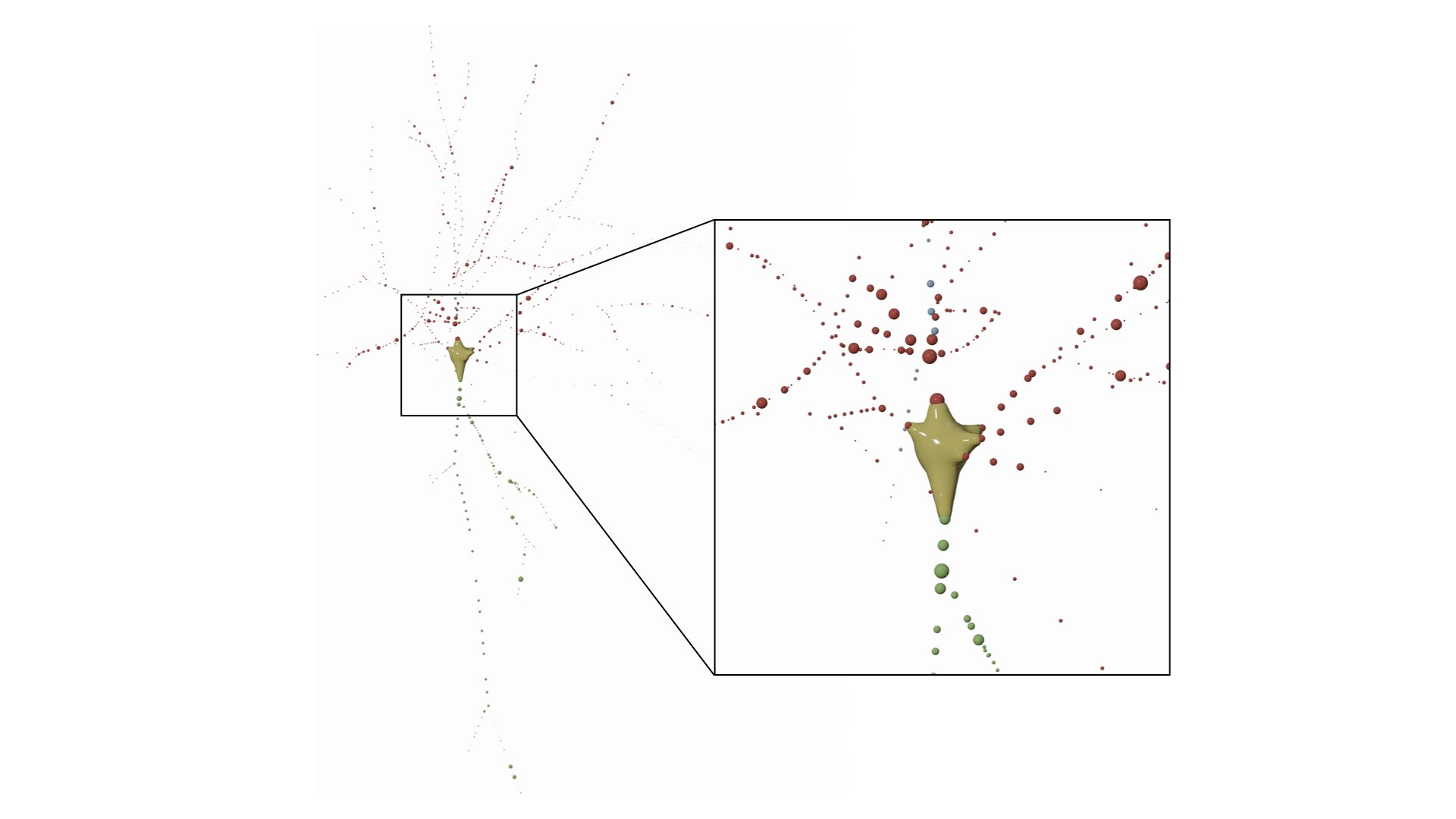
This mode can be set in the configuration file as follows:

# Morphology reconstruction method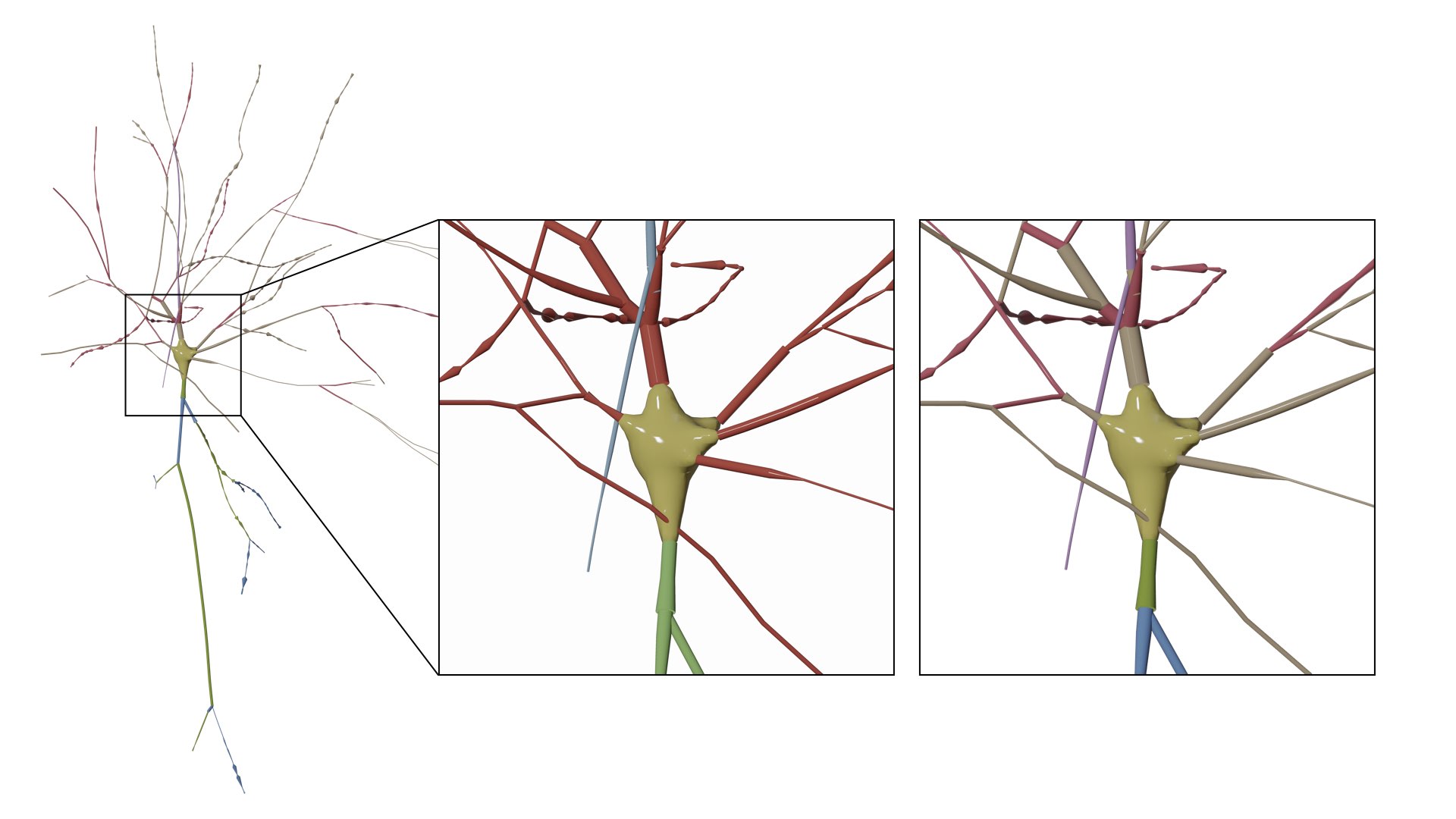
MORPHOLOGY_RECONSTRUCTION_ALGORITHM=samples

This mode draw a three-dimensional dendrogram of the morphology. Note that the subtrees are color-coded by the same colors in the morphology and dendrogram plots. These colors can be selected by the user from the Morphology Colors section in the panel before rendering the images.

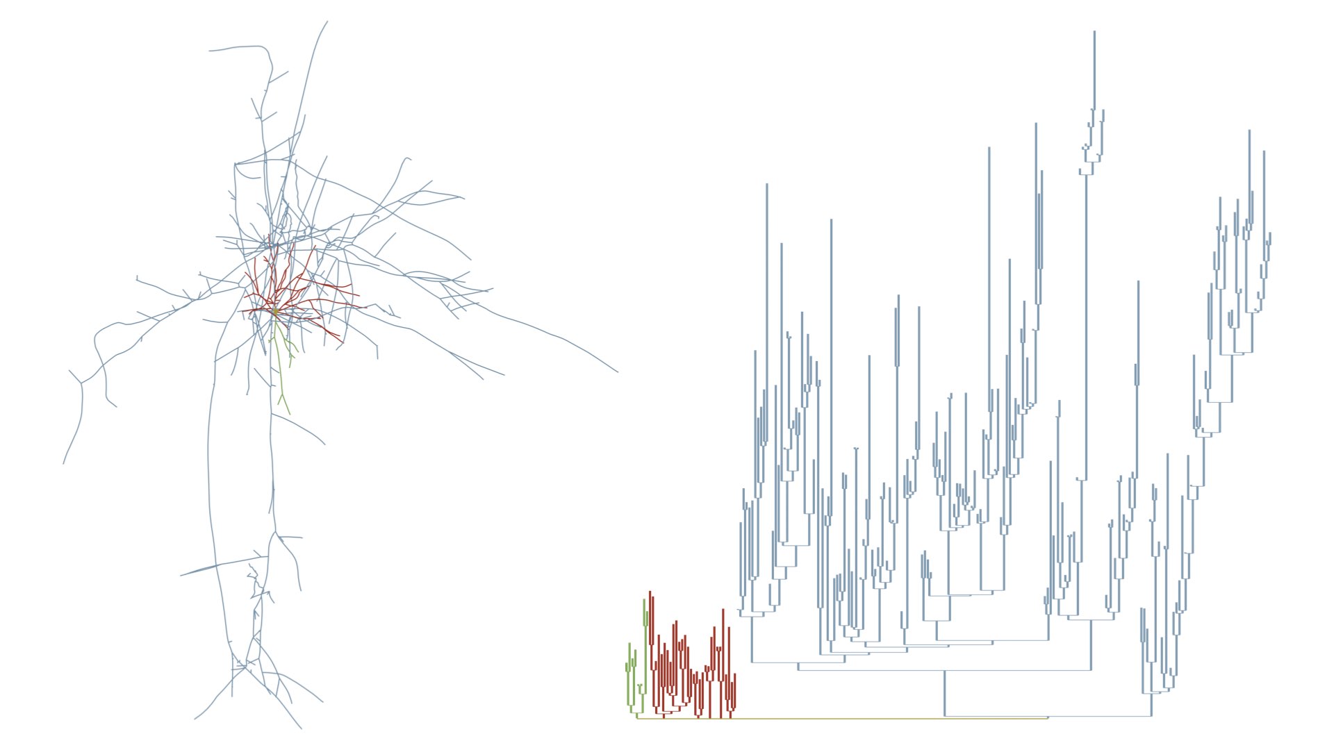
# Morphology reconstruction method
MORPHOLOGY_RECONSTRUCTION_ALGORITHM=dendrogram

• Original
• Tapered
• Zigzag
• Tapered Zigzag
• Straight

The morphology skeleton is drawn as loaded from the original file and no changes will be applied to it.

This option can be set in the configuration file as follows:

# Skeleton
SKELETON=original

Create tapered arbors where each arbor will be starting with the largest sample and terminating with the smallest sample. This mode is merely used for artistic purposes as the drawn morphology is modified from the original one.

This option can be set in the configuration file as follows:

# Skeleton
SKELETON=tapered

Create a zigzagged skeleton (to simulate the way the neurons look under the microscope when the intracellular space if filled with some stain). This style is recommended to create meshes that can be used for machine learning applications.

This option can be set in the configuration file as follows:

# Skeleton
SKELETON=zigzag

Create a skeleton with a tapered and zigzag style. Again, this option is only meant for artistic purposes as it changes the structure of the morphology.

This option can be set in the configuration file as follows:

# Skeleton
SKELETON=tapered-zigzag

Create a simplified morphology skeleton by drawing the first and last samples along each section and ignore the others.

This option can be set in the configuration file as follows:

# Skeleton
SKELETON=straight

When the Connected Sections method is used to draw the skeleton, a parent section will get connected one of the child sections starting from the root section till the leaf one. The selection of this child section can be done based on the angles between the parent and the children or the their radii.

The following branchig methods are implements:

• Angles
• Radii

Make the branching based on the angles at branching points. The parent is connected to the child with the largest angle to yield a smooth connection.

Make the branching based on the radii of the children at the branching points. The parent is connected to the child whose first sample radius is comparable.

This option defines how the arbors of the morphology will be connected to the soma when drawin the morphology.

• Connect Connected
• All Connected
• All Disconnected

Note: This option is only implemented in the GUI and cannot be set in the configuration file.

The connected arbors will be extended to the origin of the soma.

All the arbors of morphology will be extended to the origin of the soma.

All the arbors of the morphology will only be drawn starting from their the first sample of their initial segments.

The follwoing section resampling options are available:

• None
• Adaptive Relaxed
• Adaptive Packed
• Fixed Step

The resampling method can be set in the configuration file in the MORPHOLOGY/SOMA SKELETON PARAMETERS as follows:

# Skeleton Resampling
# Use ['none'] to ignore, this is the default option.
# Use ['adaptive-relaxed'] to apply adaptive resampling with relaxed distancing.
# Use ['adaptive-packed'] to apply adaptive resampling while packing each section in the morphology.
# Use ['fixed-step'] to resample the skeleton at a fixed sample step.    
MORPHOLOGY_SKELETON_RESAMPLING=none

If None is selected, the sections of the morphology will not be resampled at all and will be drawn as loaded from the morphology file.

This option can be set in the configuration file as follows:

# Skeleton resampling method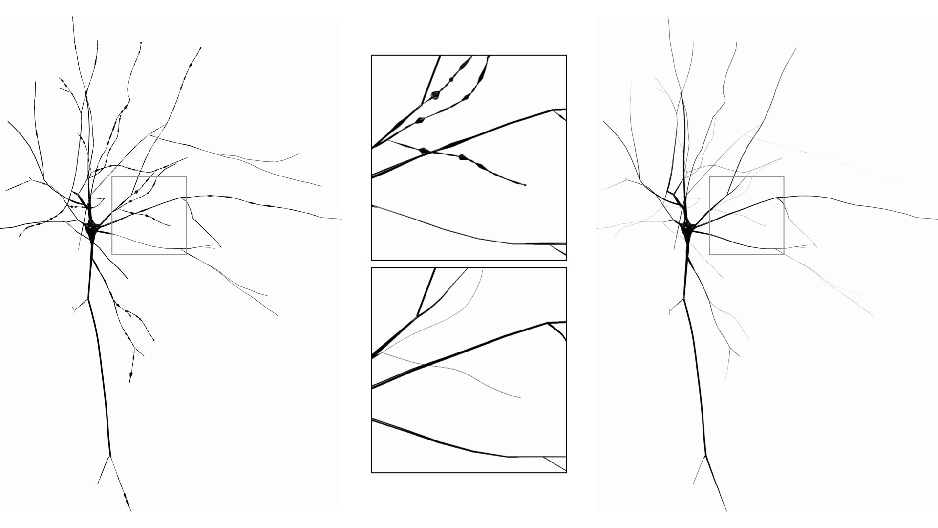 
MORPHOLOGY_SKELETON_RESAMPLING=none

Use adaptive resampling to resample each section in the morphology and remove the unwanted samples while preserving the spatial features of the section. The new samples will not be touching each other, that is why it is called relaxed.

This option can be set in the configuration file as follows:

# Skeleton resampling method
MORPHOLOGY_SKELETON_RESAMPLING=none

Use adaptive resampling to resample each section in the morphology and remove the unwanted samples while preserving the spatial features of the section. The new samples will overlap as if they pack the section to fill it entirely, and that is why it is called packed.

This option can be set in the configuration file as follows:

# Skeleton resampling method
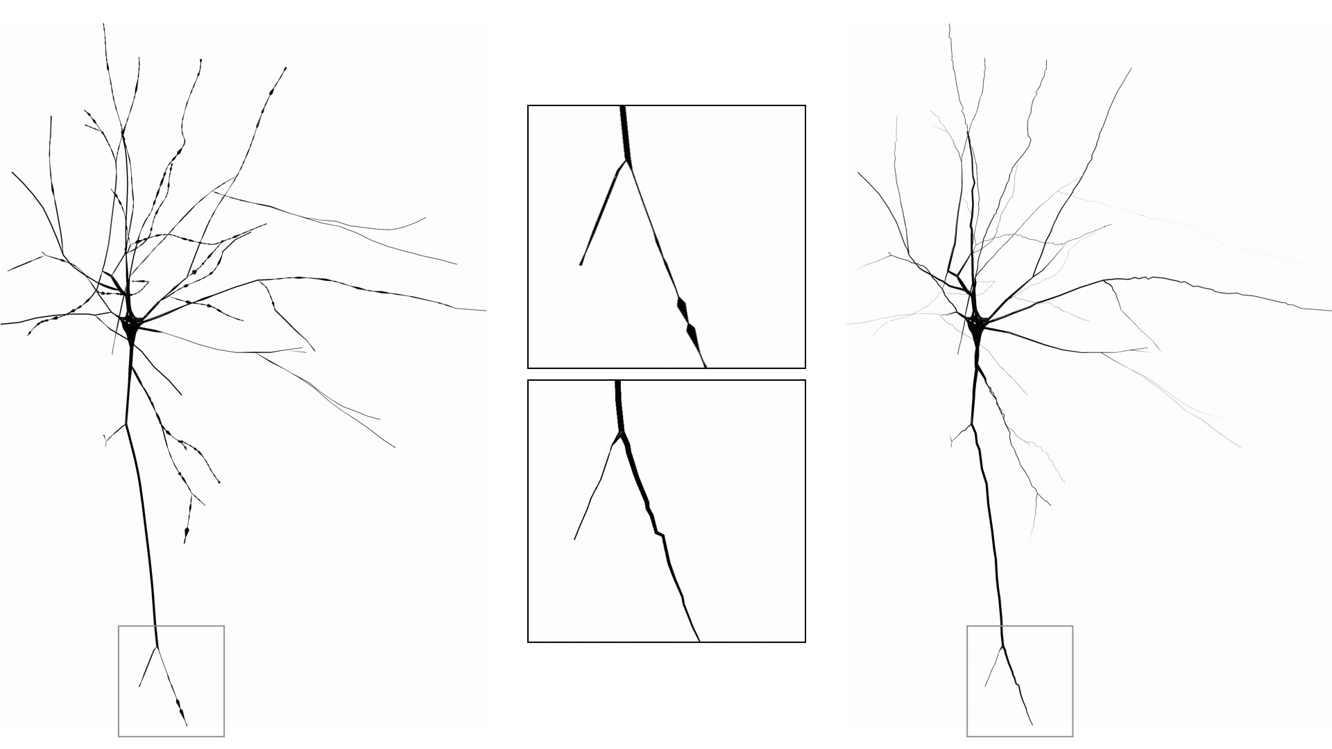
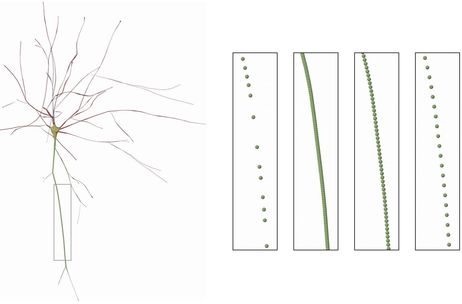
MORPHOLOGY_SKELETON_RESAMPLING=adaptive-packed

Use fixed resampling step to resample the section. With high resampling steps, some of the spatial features of the sections could be gone. If this option is selected, the user can set the step value by the Resampling Step slider which will appear following to selecting the Fixed Step option in the Resampling menu.

Resampling the skeleton at a fixed step of 1.0 will result in

If we change the fixed step to 5.0, the result will be

This option can be set in the configuration file as follows:

# Skeleton resampling method   
MORPHOLOGY_SKELETON_RESAMPLING=fixed-step

# Resampling step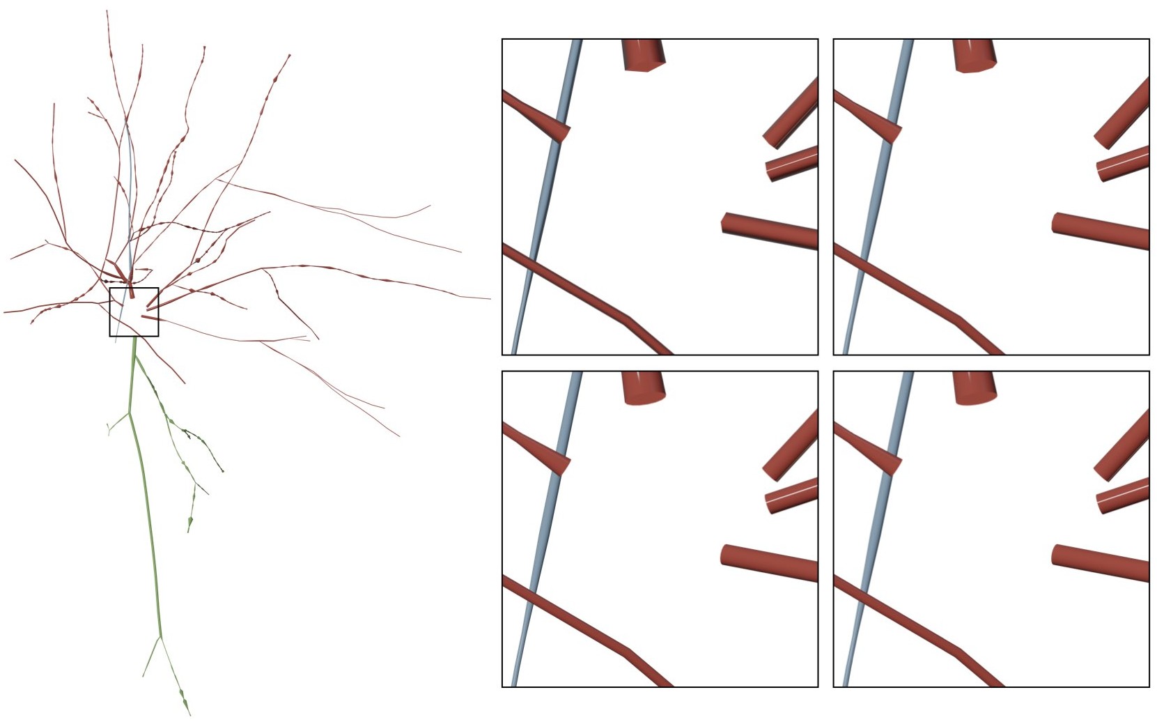
MORPHOLOGY_RESAMPLING_SETP=1.0

This option adjusts the number of sides of the bevel object used to interpolate the polylines of the morphology. By default this option is set to 16. Acceptable range for this parameter is between four and 64.

In certain cases, the radii of the morphological samples are very small or even zero. It is advisable to change the value of the actual radii to be able to visualize the morphology. The following options are available:

• Original
• Unified
• Type Unified
• Scaled

The radii of samples of the drawn skeleton will be the same as those loaded from the original morphology file.

This option can be set in the configuration file as follows:

# Section radii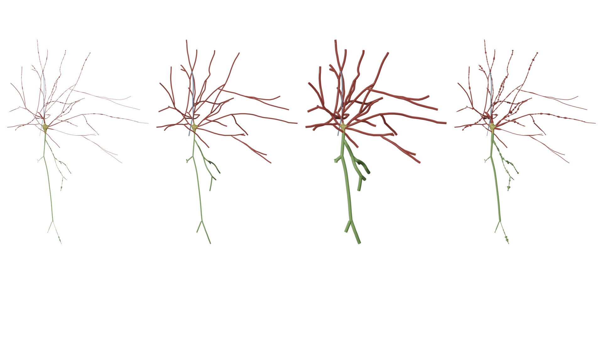 
SET_SECTION_RADII=default

The radii of all the samples in the entire morphology are set to a unified value given by the user. If this option is selected, the slider Fixed Radius Value will appear in the GUI to set the unified radius.

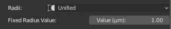
This option is very useful to visualize broken morphologies that have samples with zero radii. For example, the radius of all the samples in the morphology is set to a unified value of one as shown in the following image.

This option can be set in the configuration file as follows:

# Section radii 
SET_SECTION_RADII=fixed

# Section fixed radius value if the 'SET_SECTION_RADII=fixed' method is used, otherwise ignored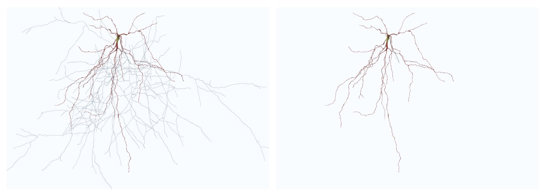
FIXED_SECTION_RADIUS=2.0

The radii of all the samples in the different branches (axon, apical dendrite and basal dendrites) will be set to unified values specific to axon, apical dendrite and basal dendrites. If this option is selected, the following sliders Axon Radius, Apical Dendrite Radius and Basal Dendrites Radius will appear in the GUI to set the unified radii of the axon, apical dendrites and basal dendrites respectively.

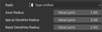
In the following example, the radii of the apical dendrite, basal dendrites and axon are set to 3.0, 2.0 and 1.0 respectively.

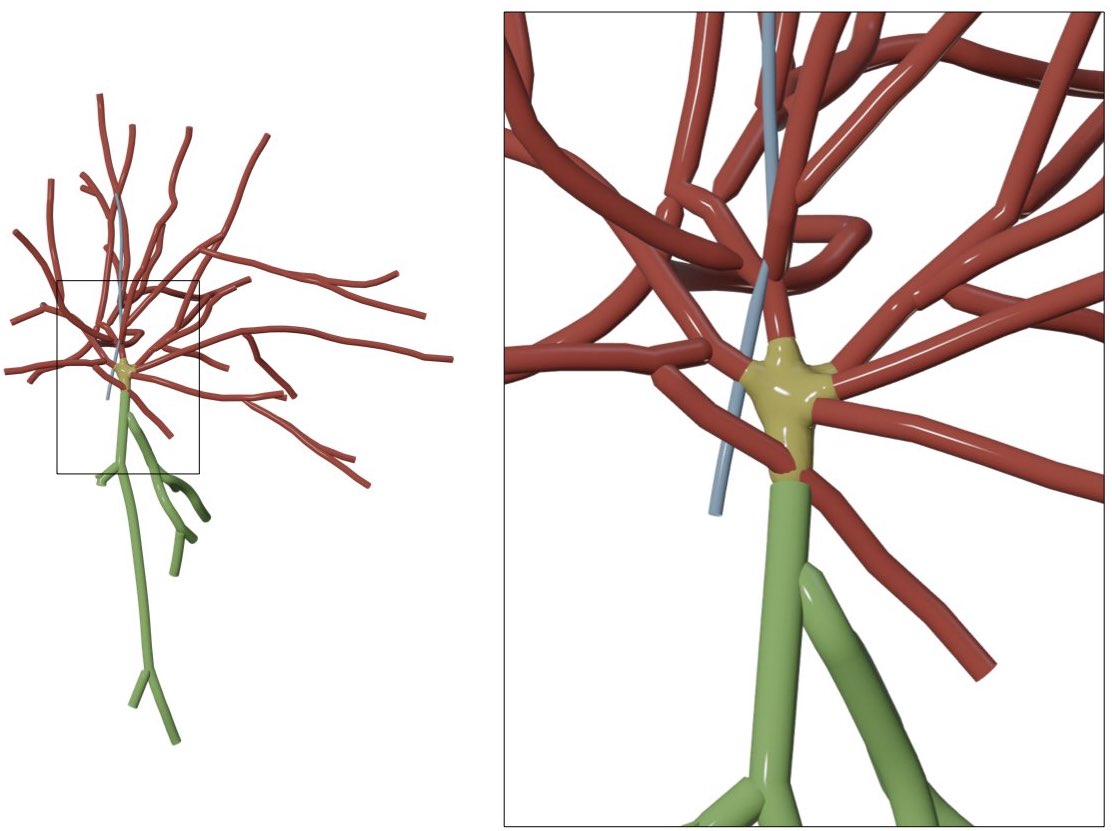
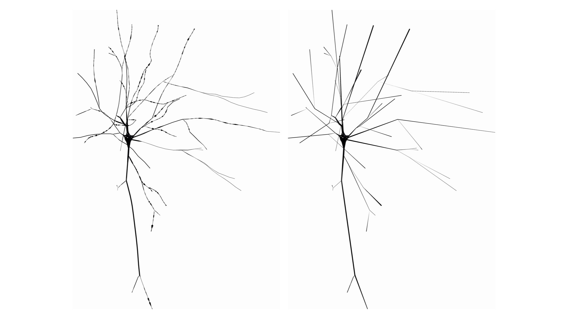
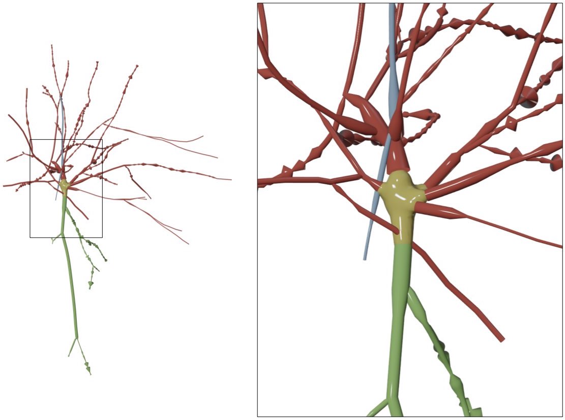
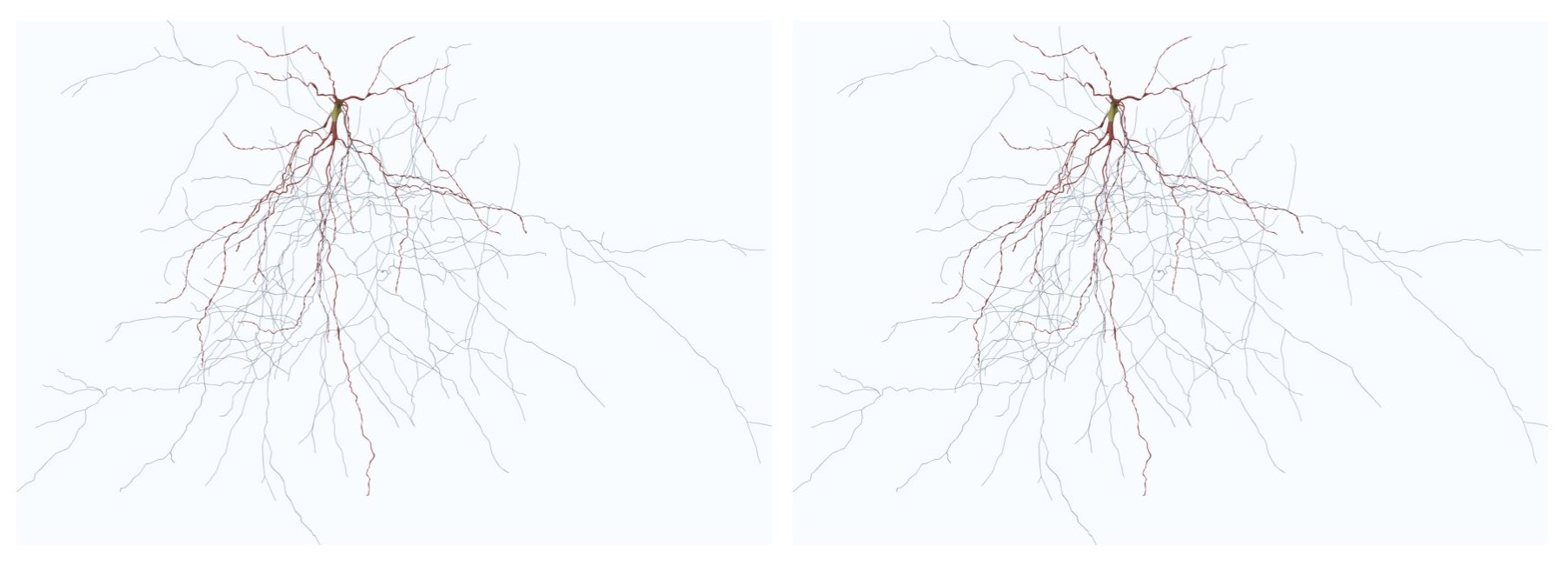
Scale the radii of all the samples in the morphology with a scale factor given by the user. If this option is selected, the slider Radius Scale Factor will appear in the GUI to set the scale factor used to scale the samples.

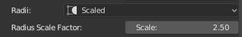
The radii of the samples in the following morphology are scaled by a 1.5 factor compared to those loaded from the original morphology file.

This option can be set in the configuration file as follows:

# Section radii 
SET_SECTION_RADII=scaled

# Radii scale factor if the 'SET_SECTION_RADII=scaled' method is used, otherwise ignored
RADII_SCALE_FACTOR=1.0

Users can select to draw the soma as a seprate object in the scene using one of the following options:

• Ignore
• Sphere
• MetaBalls
• SoftBody

Ignore the soma object and do not display it when the morphology is drawn.

Draw the soma as a symbolic sphere ceneterd at the origin.

Use the MetaBalls algotirhm to build a three-dimensional profile that approximates the soma shape. Note that the parameters of the soma can be adjusted from the Soma Reconstruction panel and they will get automatically applied while drawing the morphology.

Use the soft body physics to simulate the growth of a soma profile using the physics engine of Blender. Note that the parameters of the soma can be adjusted from the Soma Reconstruction panel and they will get automatically applied while drawing the morphology.

Users can also remove (or hide) certain branches from the visualization based on their type. We added a three checkboxes to hide/view the different components of the morphology.

• Build Axon
• Build Apical Dendrite
• Build Basal Dendrites

This options allows also the user to manually set the maximum branching order per arbor in the morphology. It is quite useful when you want to visualize the arbors till certain branching order only and ignore the rest.

Users can assign multipl shaders or materials to the different compartments of the morphologies. This includes:

• Soma Color
• Axon Color
• Basal Dendrites Color
• Apical Dendrite Color

All available shaders in NeuroMorphoVis are demonstrated in this page.

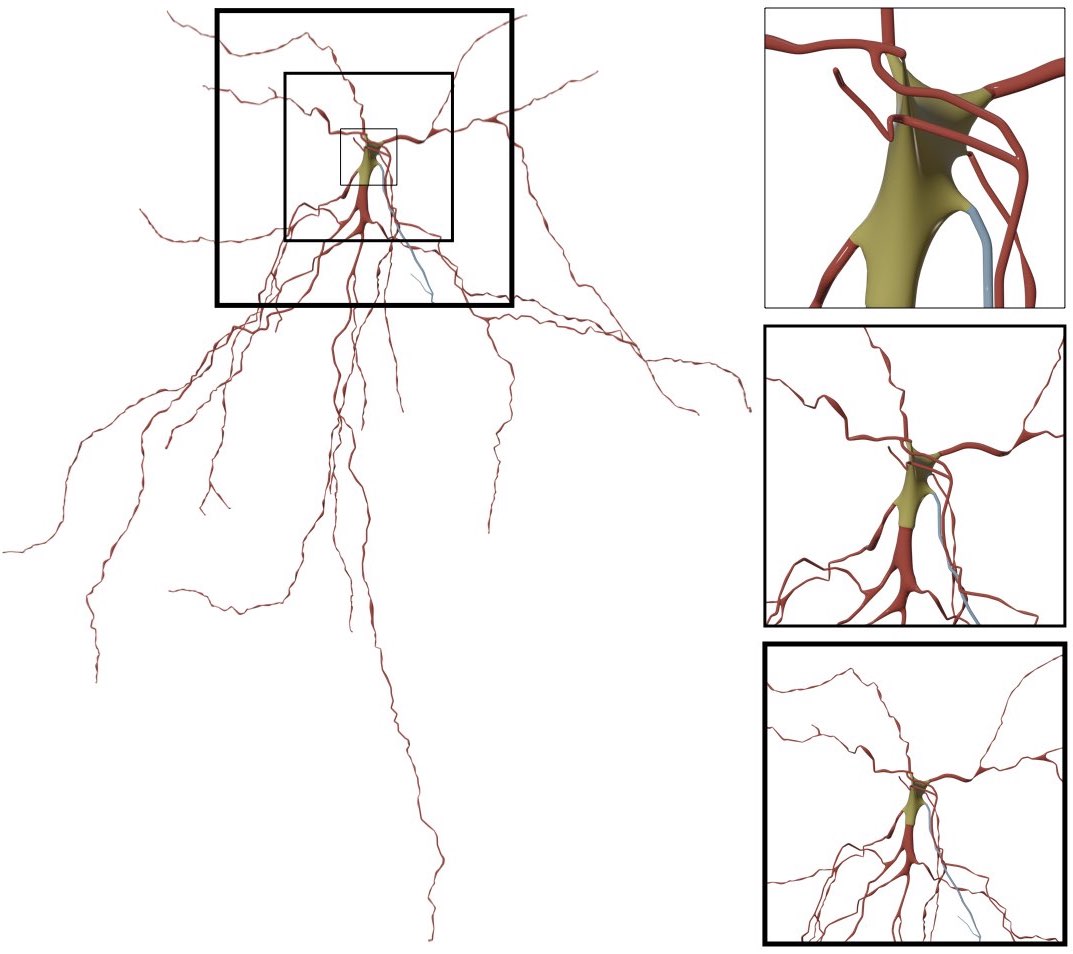
• Wide Shot
• Mid Shot
• Close Up

To understand the difference between the different shots in general, you can refer to this artlcie.

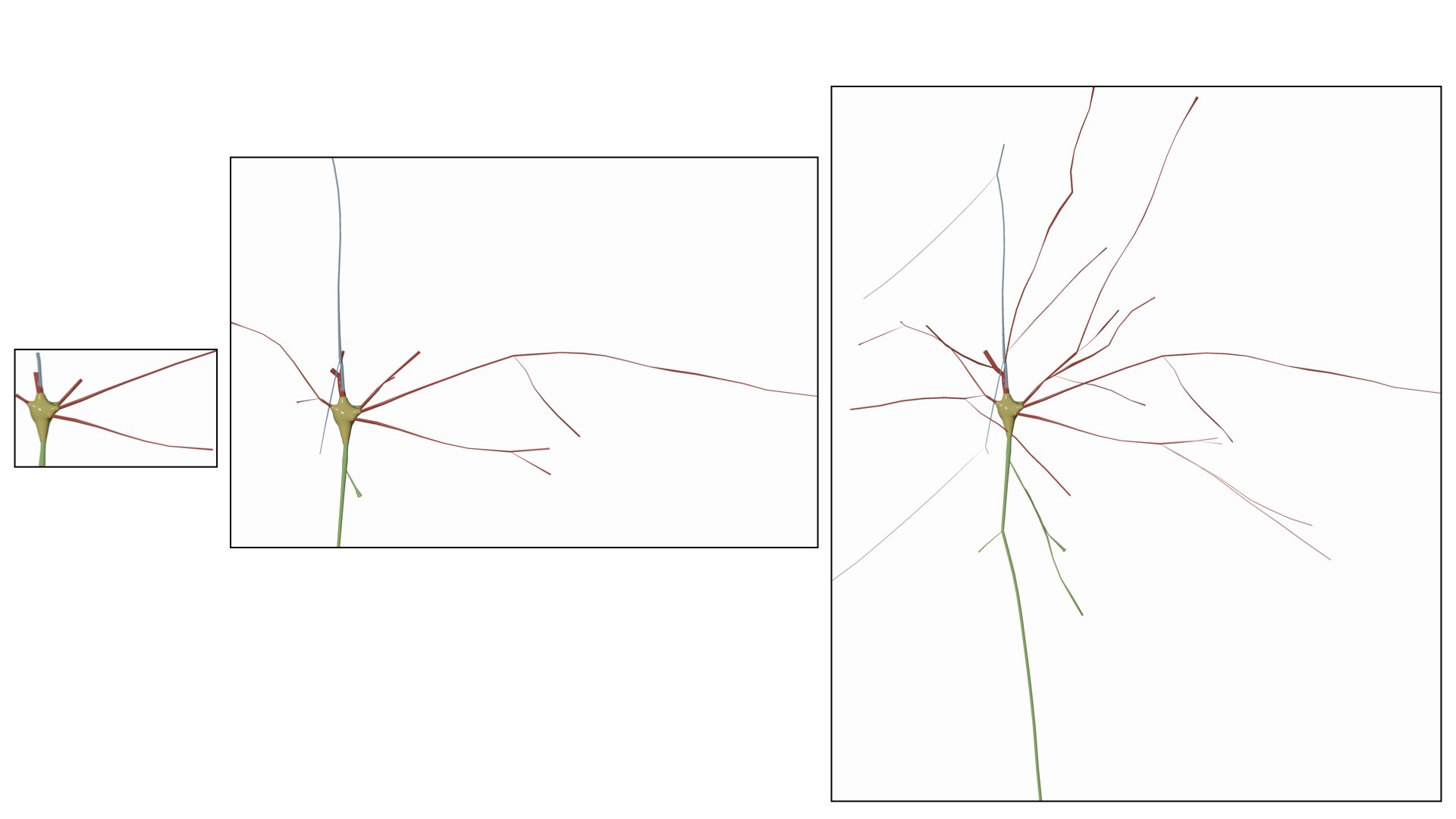
The spatial extent of a wide shot image spans that of the entire morphology, even if we limit the branching order to certain level. To render a wide shot view of the mesh, the option Wide Shot must be selected before clicking on any rendering button.

This option can be set in the configuration file as follows:

# Rendering view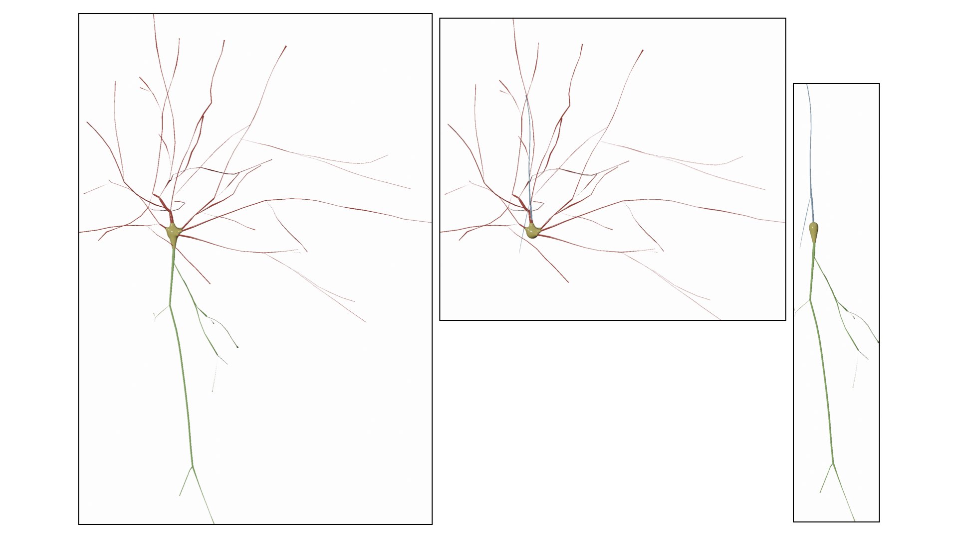 
RENDERING_VIEW=wide-shot

The spatial extent of a mid shot image is limited to the bounding box of only the arbors reconstructed at a specific branching order. To render a mid shot view of the mesh, the option Mid Shot must be selected before clicking on any rendering button.

This option can be set in the configuration file as follows:

# Rendering view 
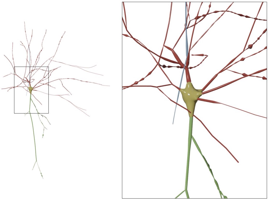
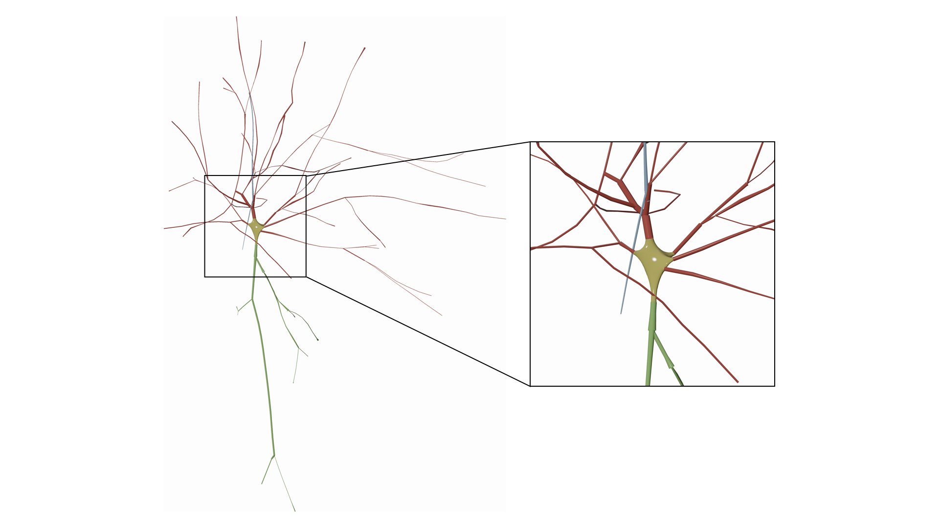
RENDERING_VIEW=mid-shot

If you select to render a closeup view of the mesh (around the soma) by clicking on the Close Up button, then you can set the size of the closeup shot in the Close Up Size field.

This option can be set in the configuration file as follows:

# Rendering view 
RENDERING_VIEW=close-up

# Close up view dimensions (in microns)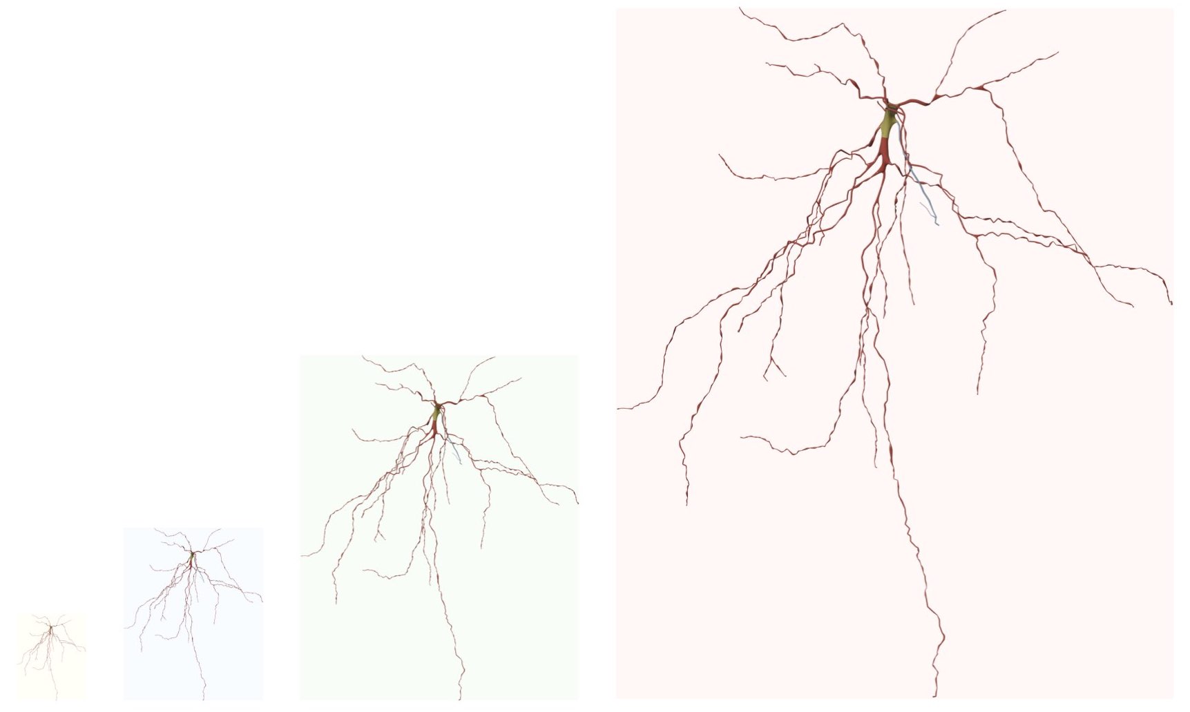
CLOSE_UP_VIEW_DIMENSIONS=20

NeuroMorphoVis has support to set the resolution of the rendered images either to a fixed resolution or based on the dimensions of the morphology skeleton. The later option is mandatory for images required for scientific articles. It allows users to render images to scale and overlay a scale bar on the top of the image.

The resolution of the image is defined by two parameters (width and height) in pixels, however, NeuroMorphoVis forces the users to define the resolution of the image using a single parameter to avoid rendering an image with distrorted aspect ratio.

This option can be set in the configuration file as follows:

# Renders a frame to scale 
RENDER_TO_SCALE=no


# Frame resolution, only used if RENDER_TO_SCALE is set to no 
FULL_VIEW_FRAME_RESOLUTION=4000

Before rendering the reconstructed mesh into an image, the three-dimensional bounding box (width, height and depth) of the mesh is automatically computed and the resolution of the image is defined based on 1) the bounding box of the mesh and 2) the rendering view. For example if the bounding box of the mesh is 100 x 200 x 300 and a front view is rendered, then the resolution of the image will be set automatically set to 100 x 200. If the side view of the mesh is rendered, then the resolution of the image will be set to 200 x 300 and finally if the top view is rendered, then the resolution of the image will be set to 300 x 100. If the user wants to render an image to scale, then option To Scale must be selected. In this case, each pixel will correspond in the image to 1 micron, and the resolution of the image is limited to the dimensions of the morphology. To render higher resolution images, however to scale, we have addedd support to scale the resolution of the image using a scale factor that is defined by the user. When the user select the To Scale option, the Scale Factor slider appears below to give the user the control to select the most approriate scale factor that fits the objective ultimate objectives of the image. By default, the scale factor is set to 1. Note that increasing the scale factor will make the rendering process taking longer O(NXM). A convenient range for the scale factor is 3-5.

This option can be set in the configuration file as follows:

# Renders a frame to scale 
RENDER_TO_SCALE=yes

# Frame scale factor (only in case of RENDER_TO_SCALE is set to yes), default 1.0
FULL_VIEW_SCALE_FACTOR=10.0

After setting all the rendering parameters as shown in the previous steps, the users can render an image of the morphology using any of the following buttons:

• Front This button renders the front view of the reconstructed morphology.

• Side This button render the side view of the reconstructed morphology.

• Top This button renders the top view of the reconstructed morphology.

This option can be set in the configuration file as follows:

# Camera view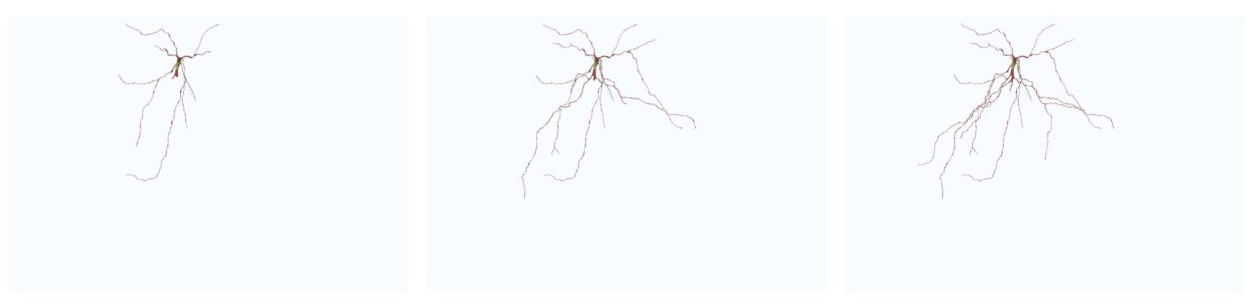
CAMERA_VIEW=front

NeuroMorphoVis has added support to render two types of movies: 360_ and Progressive sequences.

The user can render a 360 movie to visualize the morphology from different views.

# Render a 360 of the morphology, default 'no'.
# Use ['yes' or 'no']
RENDER_NEURON_MORPHOLOGY_360=yes

The user can render a progressive animation showing the progressive reconstruction (or the growth) of the morphology.

# Render the progressive reconstruction of the skeleton, default 'no'. 
# Use ['yes' or 'no']
RENDER_NEURON_MORPHOLOGY_PROGRESSIVE=yes

Users can export the drawn morphology skeleton into multiple file formats including:

• SWC (or .swc)

• Segments (or .segments)

• Blender Format (or .blend)

This is the standard file format adopted by the neuroscience community. In this format, the skeleton is represented by a list of samples, where each sample in this list has the following structure:

• The index of the sample or sample number
• The type of the sample or structure identifier
• Sample x-coordinates
• Sample y-coordinates
• Sample z-coordinates
• Sample radius
• The index of the parent sample

For further details about this format, you can refer to this link.

To export the morphology into a .swc file, click on the SWC (.swc) button under the Save Morphology As section.

The morphology file can be exported into an ASCII text file with .segments extention. This file is a list of segments. Each line in the file is a segment composed of two points between brackets. Each point has the following structure [X Y Z RADIUS]. This file is used to make it easy for other visualization application (for example to render the morphology with signed distance fields) without implementing any specific parsers.

The structure of a .segments file with 100 segments looks like this:

[X0 Y0 Z0 R0][X1 Y1 Z1 R1]
[X1 Y1 Z1 R1][X2 Y2 Z2 R2]
[X2 Y2 Z2 R2][X3 Y3 Z3 R3]
...
...
...
[X99 Y99 Z99 R99][X100 Y100 Z100 R100]

An example of this file is available in this link.

To export the morphology into a .segments file, click on the Segment (.segments) button under the Save Morphology As section.

To export the morphology into a .blend file, click on the Blender Format (.blend) button under the Save Morphology As section.

Note The saved file must be opened with the same Blender version used to export the file. If the file is saved with Blender 2.7, you can load it with Blender 2.8 but not vice verse.

• Starting

  • Home
  • Downlading NeuroMorphoVis
  • Installing NeuroMorphoVis
  • Running NeuroMorphoVis
  • FAQs

• Panels

  • Input / Output
  • Morphology Analysis
  • Morphology Editing
  • Soma Reconstruction
  • Morphology Reconstruction
  • Synaptics
  • Mesh Reconstruction
  • About NeuroMorphoVis

• Other Links

  • Analysis Kernels
  • Colors & Shading
  • Configuration File