Running OpenXY - BYU-MicrostructureOfMaterials/OpenXY GitHub Wiki

For installation instructions click here.

Contents

• Instructions:
  • Overview of Running OpenXY
  • Detailed Instructions on Running OpenXY
• Explanation of individual Graphical User Interfaces (GUIs)
  • MainGUI
  • Advanced Settings GUI
  • ROI Settings GUI
  • Microscope Settings GUI
  • PC Calibration GUI
  • Output Plotting GUI

Overview of Running OpenXY

These are the basic steps of the analysis procedure:

1. Select Scan and first image
2. Edit options with the settings menus (Optional)
3. Perform Cross-Correlation Analysis/ Dislocation Density Calculation
4. Plot Results

Detailed Instructions on Running OpenXY

These instructions assume a basic understanding of Matlab functionality.

1. Open and Run RunOpenXY.m (calls MainGUI.m) in Matlab (accept any prompt to change folder)
2. Select the scan file (.ang or .ctf)
   • If a .ang file is selected, OpenXY attempts to find a Type I grain file (.txt) with the same name in the same directory. If none is found, it will prompt the user to select the grain file. Currently only Type I grain files are supported.
   • If a .ctf file is selected, OpenXY attempts to find a .cpr file with the same name in the same directory. If none is found, it will cause an error.
3. Select the first image in the scan
   • All images files supported by the Matlab imread.m function are supported by OpenXY. This includes .jpg, .tiff, .bmp, .png, and .gif formats.
4. Set the output file
   • The name of actual outputs will have prefixes added to this name (see info window below button).
   • OpenXY will automatically check if any files will be overwritten.
5. Change microscope settings
   • Open microscope settings from Settings|Microscope Settings menu (or press Ctrl+M).
   • Change microscope settings to match the the scan.
   • For more information on microscope settings click here
6. Change Calculation Preferences
   • Open advanced settings from Settings|Advanced Settings (or press Ctrl+A).
   • For more info on the advanced settings menu click here
7. Change ROI/Image Preferences
   • Open ROI settings menu from Settings|ROI Settings (or press Ctrl+R)
   • For more info on the ROI Settings menu click here
8. Edit the Pattern Center calibrations
   • Open ROI settings menu from Settings|PC Calibration (or press Ctrl+X)
   • For more info on PC Calibration click here
9. Select Scan Type
   • Use "Scan Type" dropdown menu on MainGUI
   • Both Square and Hexagonal scans supported
   • Select Square scan type for line scans
10. Select Material

• Use "Material" dropdown menu on MainGUI
• Manually select from the list of materials OR
• Set to “Scan File” to use the material specified in the scan file
• For info on adding/editing a material, click here

11. Select Number of Processors

• Use "Processors" dropdown menu on MainGUI
• Defaults to one less than the total number of processor cores available
• OpenXY detects the number of processor cores available for parallel processing (logical cores not included)
• Select 1 core to disable parallel processing, and select more cores for faster calculation time

12. Enable/Disable Display Shifts

• Check the "Display Shifts" box to enable output of Strain Tensor to command window and display the shifts plotted on the reference and experimental image through each cross-correlation iteration
• For more information, click here

13. Run OpenXY

• Select the green "Run" button on MainGUI to start the cross-correlation analysis
• PC Calibration will appear if selected

14. Display Results

• The Output Plotting window will appear upon completion of the analysis
• Generate plots from list of available parameters
• For more info on Output Plotting click here

MainGUI

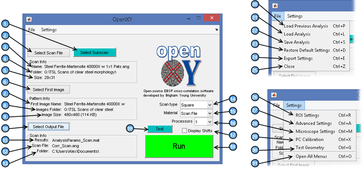
1. Select Subscan: Opens a menu alowing you to selct a smaller sub-scan to run cross-correlation analysis on.
2. Select Scan File: Opens a window to select a .ang or .ctf fie. Automatically checks for the corresponding grain or .cpr file. Will display a warning message if none is found.
3. Once a file is selected using (2), the name of the scan file is displayed
4. Once a file is selected using (2), the folder of the scan file is displayed
5. Once a file is selected using (2), the size (rows x columns) of the scan is displayed
6. Select First Image: Opens a window to select the first image in the scan. All image types supported by the Matlab imread function are supported (includes .jpg, .tiff, .bmp, .gif, and .png). OpenXY will automatically attempt to verify if the image is the first image in the scan, and will query the user if a discrepancy is found.
7. Once an image is selected using (6), the name of the image is displayed
8. Once an image is selected using (6), the folder of images is displayed
9. Once an image is selected using (6), the size of the image is displayed [pixel height x pixel width (size in KB)]
10. Select Output File: Opens a window to select the location and base name of the output files. Automatically checks if any files will be overwritten
11. Once a file is selected using (10), the name of the results file (.mat) is displayed. "AnalysisParams_" is appended to the name specified in (9)
12. Once a file is selected using (10), the name of the corrected scan file (.ang or .ctf) is displayed. "Corr_" is appended to the name specified in (9)
13. Once a file is selected using (10), the output folder is displayed
14. Scan Type: Specifies the layout of the points of the scan. Select "Square" for a linearly aligned grid. Select "Hexagonal" for an offset grid pattern. Select "Square" for line scans.
15. Material: Select the material of scan. Select "Auto-detect" prior to selecting the scan file in (2) to allow OpenXY to attempt to identify the material from the grain or .cpr file. For more information on adding or editing materials click here
16. Processors: Specifies the number of cores assigned the Matlab Parallel Processing pool. Defaults to one less than the total number of cores (not including logical cores) available. Select 1 core to disable parallel processing (for now, the parallel processing toolbox is still required).
17. Display Shifts: Displays graphical representation of regions of interest (ROI) shifts during cross correlation. Not available with parallel processing, select 1 processor (16) to enable. For more information, click here.
18. Run Button: Starts cross-correlation analysis. The analysis steps are outlined below:
19. Extract information from scan file, correlate each point with an image file, and set up key variables.
20. Perform cross-correlation using real or simulated reference images
21. Calculated dislocation density (optional)
22. Launch Output Plotting GUI
23. Test: Perform cross-correlation on a single image of the scan.
24. Load Previous Analysis: Loads previous settings from previous session. May not load any settings if no settings were selected the last time MainGUI was launched.
25. Load Analysis: Loads settings saved in a .mat file. File must contain a Settings structure. The output (AnalysisParams_...mat) file of a previous analysis may be selected to load the settings used in that analysis.
26. Save Analysis: Saves current settings to a .mat file that may be reloaded later
27. Restore Default Settings: Restores all settings to their initial settings when MainGUI is launched. This includes the scan, image, and output file selections.
28. Esport Settings: Exports the current settings to the MatLab workspace.
29. Close: Exits MainGUI and saves current settings to a temporary file (may be reloaded by (19))
30. ROI Settings: Launches ROI Settings GUI to edit image filter and ROI selection settings. For more information click here.
31. Advanced Settings: Launches Advanced Settings GUI to edit calculation options such as reference pattern type (real or simulated) and enable dislocation density calculation. For more information click here.
32. Microscope Settings: Launches Microscope Settings GUI to edit microscope settings such as acceleration voltage and sample title. For more information click here.
33. PC Calibration: Launches PC Calibration GUI. Uses strain minimization to correct the pattern center for each point of the scan, improving the accuracy of the strain calculation. More information coming soon.
34. Test Geometry: Launches the Test Geometry GUI to test the accuracy of the geometry calibrations for the scan. More information coming soon.
35. Open All Menus: Opens all menu GUIs.

Display Shifts

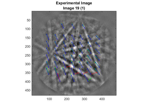
This option will display each image of the scan alongside the corresponding reference image. On top of these images will be the calculated shifts of each of the ROIs. The green lines represent the shifts that are used to calculate the deformation gradient tensor, while the red ones are outliers that are ignored in the calculation. Outliers are determined according to the Standard Deviation option (4) in Advanced Settings. The blue lines are the shifts predicted by the final deformation gradient tensor.

Advanced Settings

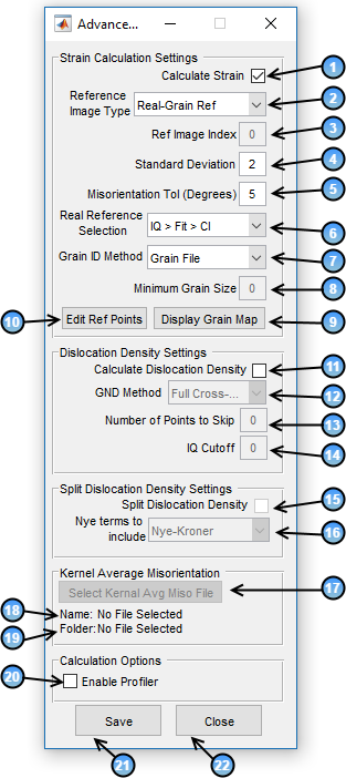
1. Calculate Strain: Toggles whether or not strain is calculated when cross corelation is run.
2. Reference Image Type: Specifies the type and location of the reference images used in the cross-correlation analysis
   • Simulated-Kinematic: Kinematically simulated patterns. Allows for absolute strain measurement.
   • Simulated-Dynamic: Dynamically simulated Patterns. Allows for absolute strain measurement. Note: Requires EMsoft. For information on installing EMsoft, click here.
   • Real-Grain Ref: Selects a single reference pattern from a central position in each grain. Enables (10)
   • Real-Single Ref: User selects a reference image in (3) using the image's index ((3) will change from "Iteration Limit" to "Ref Image Index" when a Real reference pattern method is selected.)
3. Iteration Limit OR Ref Image Index:
   • Iteration Limit: Specifies the number times the analysis will loop through the cross-correlation algorithm. For more information on the calculation click here
   • Ref Image Index: For "Real-Single Ref" selection in (1), selects the image to be used as the reference pattern for the entire scan.
4. Standard Deviation: Specifies the number of standard deviations of error to determine outlier ROI shifts to be removed. Typical values are between 2-4.
5. Misorientation Tol (Degrees):
6. Real Reference Selection:
   • IQ > Fit > Cl:
   • Min Kernel Avg Miso: Enables (17)
7. Grain ID Method:
   • Grain File: Use the grain information in the grain file.
   • Find Grains: OpenXY manually locates grains. Enables (8)
8. Minimum Grain Size: Determines the minimum size of each grain when the Find Grains option is used.
9. Display Grain Map: Displays a plot representing the individual grains in the scan.
10. Edit Ref Points: Edit the points used as reference images when Real-Grain Ref option is used.
11. Calculated Dislocation Density: Check to enable dislocation density calculation. Will add an alpha_data structure to output file containing dislocation density data. Enables (12)-(13).
12. GND Method:** Selects which method is used to calculate dislocation density:

• Full Cross-Correlation:
• Partial Cross-Correlation: Strain must also be calculated with this option.
• Orientation-Based:

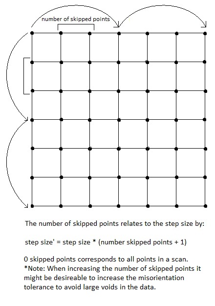
13. Number of Points to Skip: 3 options

• 'a': Runs all step sizes
• 't': Run step sizes of 2
• Positive integer: Number of points to skip

14. IQ Cutoff:
15. Split Dislocation Density: Enables (16)
16. Nye terms to include:

• Nye-Kroner:
• Nye-Kroner (Pantleon):
• Distortion-Matching:

17. Select Kernal Avg Miso File:
18. Displays the name of the selected file.
19. Displays the folder where the selected file is saved.
20. Enable Profiler: Runs a Profiler during cross corelation and displays the results after analysis is completed.
21. Save & Close: Saves all changes.
22. Cancel: Discards all unsaved changes and returns to MainGUI.

ROI Settings

The ROI Settings menu can only be opened once a scan file and first image have been selected in MainGUI

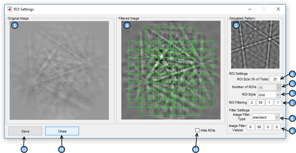
1. Original Image: Original EBSD image without any filters or alterations. Will be cropped to a square.
2. Filtered Image: EBSD image after filter values (9) are applied. Can be refreshed using (12)
3. Simulated Pattern: Equivalent Simulated Pattern for the first image. Use Filtering (9) to change filters
4. ROI Size: Size of each ROI in percent of entire image
5. Number of ROI's:* Number of ROI's used in cross-correlation
6. ROI Style: 3 Options
   • Grid: Fixed number of ROIs at fixed locations on image arranged in a grid pattern. Uses a fixed ROI count (4) of 48.
   • Radial: ROI's arranged in two rings about the center of the image.
   • Intensity: Centers each ROI on "bright spots" on the image. Currently not functioning.
   • Annular: ROI's arranged in a rings about the center of the image.
7. ROI Filtering: 1x4 numeric vector: [lower radius (pixels), upper radius, smooth lower radius filter switch, smooth upper radius filter switch]. Used in CalcF.m for error function filter. Filtered by custffx.m. If smooth switches are off, it cuts out high and low frequencies in FFT space; if switches are on it smooths the interface at the cut-offs.
8. Image Filter Type: 2 Options
   • Standard:
   • local thresh:
9. Image Filter Values: Same as ROIFilter (7), but for entire image. Called in GetDefGradientTensor.m to ReadEBSDImage.m to custimfilt.m.
10. Hide ROIs: Stops displaying the ROIs on the filtered image (2).
11. Save: Saves all changes made.
12. Close: Discards all unsaved changes and returns to MainGUI.

Microscope Settings

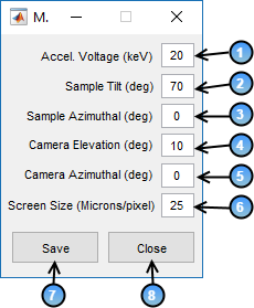
1. Accel Voltage: The strength of the electron beam set by the user in the SEM, in KeV.​
2. Sample Tilt: The inclination of sample surface with respect to the perpendicular to the electron beam. 70 deg is considered ideal for EBSP collection. The angle is converted to radians when stored in the code.
3. Sample Azimuthal: The anticlockwise angle between the positive x-axis of the phosphorus screen and the projection of the normal vector of the sample onto the xy plane of the phosphorus screen.
4. Camera Elevation (deg): The inclination of the camera normal to the horizontal.
5. Camera Azimuthal (deg): The anticlockwise angle between the positive x-axis of the phosphorus screen and the projection of the normal vector of the camera onto the xy plane of the phosphorus screen.
6. Screen Size: The scale of the scans in microns/pixel.
7. Close: Discards any unsaved changes and closes the GUI.
8. Save: Saves the current settings.

PC Calibration

Uses strain minimization on a number of selected points to correct the pattern center for each point in the scan. Allows for a couple plane fitting options.

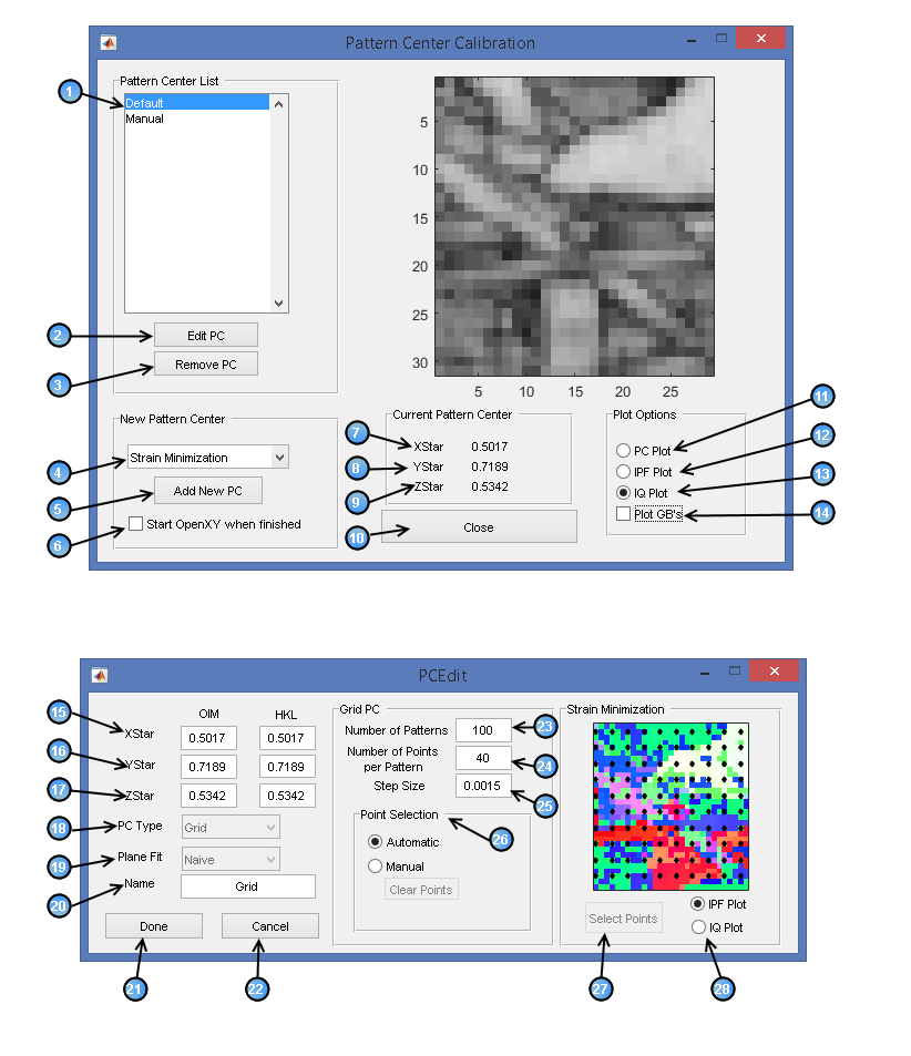
1. Pattern Center List: Lists of pattern center calibrations.
2. Edit PC: Opens the PCEdit GUI to edit the currently selected Pattern center calibration.
3. Remove PC: Delete currently selected pater center calibration.
4. Pattern Center Type: Choose the type of calculation to compute the new pattern center. You can choose from the following options:

• Strain Minimization:
• Grid:
• Manual: Manually enter the position of the pattern center.

5. Add New PC: Opens the PCEdit GUI to adjust settings to create a new pattern center calibration, then runs the calculations. Note: this process can take several hours.
6. Auto-Run OpenXY: If this box is checked when Add new PC is selected, OpenXY will automatically run after pattern center calculations are complete.
7. X Star: The x coordinate of the pattern center.
8. Y Star: The y coordinate of the pattern center.
9. Z Star: The z coordinate of the pattern center.
10. Close: Closes the PCGUI and returns to the MainGUI.
11. PC Plot: Plots the Default pattern center, the new pattern center and the pattern center adjustment plane.
12. IPF Plot: Plots the inverse pole figures for the entire scan.
13. IQ Plot: Plots the image quality for the entire scan.
14. Plot GB's If this box is checked, will also plot the grain boundaries. Note: Not available with PC Plot.
15. X Star: Enter the coordinate for X star. Will automatically convert between OIM & HKL.
16. Y Star: Enter the coordinate for Y star. Will automatically convert between OIM & HKL.
17. Z Star: Enter the coordinate for Z star. Will automatically convert between OIM & HKL.
18. PC type: Select the type of pattern center calibration.
19. Plane Fit: Select the type of plane fit.
20. Name: Name this pattern center calibration.
21. Done: Close the PCEdit GUI and either save the changes or begin pattern center calculations.
22. Cancel: Close the PCEdit GUI without either saving the changes or beginning pattern center calculations.
23. Number of Patterns: Enter the number of patterns used in pattern center calibration.
24. Number of Points per Pattern: Enter the number of points per pattern.
25. Step Size: The size of steps taken
26. Point Selection:

• Automatic: Automatically arranges the points in a square grid.
• Manual: Allows the user to manually select points used in the pattern center calibration.

21. Select Points: Displays a plot that allows the user to select the points used in pattern center calibration.
22. Plot Type:

• Inverse Pole Figure: Displays the inverse pole figure plot of the scan.
• Image Quality Figure: Displays the image quality plot of the scan.

Output Plotting

Generates several plots for displaying results from OpenXY

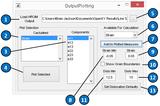
1. Load HROIM Output: File name and path of AnalysisParams_...mat results file being analyzed. Selected using (5).
2. Calculated: List of parameters being analyzed. Selected using (6) and (7). Double-click to remove parameters and any corresponding components in (3).
3. Components: Individual components (plots) of calculated parameters listed in (2). Double-click to remove from the list.
4. Plot Selected: Plot all selected calculations (2) and their corresponding components (3)
5. Select Results File: Opens a window to select an AnalysisParams_...mat results file. Must contain the Settings structure. Must contain analysis_params structure to plot dislocation density. Will auto-detect line scans and add options to generate line-scan-specific plots.
6. Available for Calculation: Drop-down menu with available plots, depending on what you chose to compute in Advanced Settings:
   • Strain: Generates 6 plots of individual strain components
   • Dislocation Density: Generates 4 plots of dislocation density: 3 plots of individual components and 1 total.
   • Split Dislocation Density:
   • Tetragonality: Not currently available
   • Line Scan Plots: Generates line plots of individual strain components and a separate plot of tetragonality.
7. Add to Plotted Measures: Adds currently selected calculation in (6) to (2) and (3)
8. Strain Min: Minimum value of strain axis in strain plots
9. Strain Max: Maximum value of strain axis in strain plots
10. Show Grain Boundaries: Plots he grain boundaries on top of the selected plot methods.

• Note: 11-12 only available if dislocation density was computed during cross-correlation.

11. Dislo Min: Minimum value of the dislocation axis in dislocation density plots
12. Dislo Max: Maximum value of the dislocation axis in dislocation density plots
13. Set Dislocation Defaults: Calculates (11) and (12) based on data.