DETECTED_OUTLIER_JACKKNIFE - AtlasOfLivingAustralia/ala-dataquality GitHub Wiki
This assertion (issue) is not supported in ALA pipelines processing, June 2021
Outlier information is supported in the fields:
- outlierLayer - identifying a record as an outlier for a layer
- outlierLayerCount - the record is identified as an outlier in this number of layers
These fields are available in the facet filtering. See this article for information on facet filtering: https://support.ala.org.au/en/support/solutions/articles/6000249564-how-to-use-facets-to-filter-ala-data
| Name | DETECTED_OUTLIER_JACKKNIFE |
|---|---|
| Code | 38 |
| Description | The location is an outlier detected using reverse jack-knife algorithm |
| Severity/Verification/Metric | Error |
| Failure implication | Optionally exclude from mapping and other reports |
| Darwin Core Class | Location |
| Darwin Core Fields | decimalLongitude, decimalLatitude |
| New/Currently Supported | New |
References
Barnett, V. and T. Lewis 1979. Outliers in Statistical Data. John Wiley and Sons. p.365.
Chapman, A.D. 1999. Quality Control and Validation of Point-sourced Environmental Resource Data. in Lowell, K. and Jaton, A. eds. Spatial Accuracy assessment: Land information uncertainty in natural resources. Chelsea, MI: Ann Arbor Press. Explains the original algorithm.
Chapman, A.D. 2005. Principles and methods of Data Cleaning - Primary Species and Species-Occurrence Data, Version 1.0. Report for Global Biodiversity Information Facility, Copenhagen. Explains the updated algorithm.
Hijmans, R. Online. DIVA-GIS http://www.diva-gis.org/ The most refined implementation of the algorithm.
Implementation notes (algorithms)
This is a well established method originally developed in ERIN, but applied elsewhere. The Reverse Jackknife method is described by Chapman A.D. 2005. Principles and Methods of Data Cleaning - Primary Species and Species-Occurrence Data,(http://www.gbif.org/orc/?doc_id=1262) who mentions that it has proved extremely reliable in automatically identifying suspect records, with a high proportion (around 90%) of those identified as being suspect, proving to be true errors. The algorithm is summarised on page 51 of the report, and is is based on a method described by Barnett and Lewis (1978). The expression is represented thus:
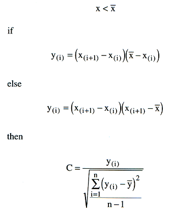
The threshold value curve has the formula t = (0.95 x sqrt(n))+0.2. The Diva implementation further adds t = t x range / 50.
The jackknife method works by first calculating the sample mean, standard deviation and range; and then steps through the sorted values comparing the distance to the mean of it and the next value. Where the distance to mean between values is above a threshold level then that sample value and those further away from the mean are flagged as outliers. An outlierness metric is also calculated for the sample value.
The algorithm is typically implemented using a set of species occurrence locations (decimalLongitude, decimalLatitude) and sample values derived from one or more environmental surface grids (e.g. climate surfaces, or latitude, longitude and elevation). Note that (i) duplicate species location coordinates are normally removed from the location dataset; and (ii) the method is only suited for use with continuous numerical environmental surface data which varies relatively gradually over geographic landscape; and is not suited to discrete or categorical environmental data.
Outlier metrics that can be derived are (i) the frequency of environmental surface grids for which the location was flagged as an outlier; and (ii) the outlierness metric.
There are a number of implementations of the algorithm, for example (i) Diva GIS http://www.diva-gis.org/, see source code example at http://www.diva-gis.org/node/111, and (ii) CRIA http://www.cria.org.br/~renato/temp/bg_report.html with source code at http://sourceforge.net/projects/gbif/files/Data%20Tester/0.2/
There are a number of differences in the two implementations of the algorithm:
Calculating Threshhold Value (t): CRIA calculates t using the expression as originally implemented: t = (0.95 x sqrt(n))+0.2. While, the Diva implementation further adds t = t x range / 50.
Calculating Sample Statistics: Having removed duplicate locations, the Diva implementation calculates the sample statistics (mean and standard deviation and number of samples) for the entire set of derived environmental values. The CRIA/GBIF implementation makes a unique set of derived sample values by discarding duplicate values and calculates the sample statistics from the generally fewer values, causing n to diminish and also affecting statistics, e.g.
| version | surface | n | mean | std | min | max | range | original samples |
|---|---|---|---|---|---|---|---|---|
| Diva | aus_100p1e | 1742 | 15.21944 | 1.513257 | 10.4 | 17.7 | 7.3 | 1742 |
| CRIA | aus_100p1e | 78 | 14.24919 | 2.118768 | 10.4 | 17.7 | 7.3 | 1742 |
Also the CRIA implementation optionally excludes zero values, while Diva always includes them.
The Diva method has been extensively tested and should be utilized in the first instance. Further investigation could be undertaken to test the CRIA variant with a view to including it as an option.
A python work bench has been established at the ALA to allow development of data quality check methodologies. Below are several example plots from the workbench:
Figure 1
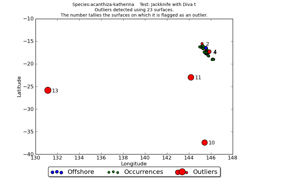 Figure 1 shows the overall results of applying the jackknife test to 23 surfaces: (latitude, longitude, elevation and 20 climate surfaces) to occurrences of the Acanthiza katherina Mountain Thornbill, an inhabitant of upland rainforest in north-eastern Queensland. Detected outlier values are shown in red with the number of surfaces for which it was an outlier indicated. Occurrences falling in the sea are shown in blue. The plot indicates three obviously erroneous to the south west of the core range, along with number of local scale potential outliers requiring investigation.
Figure 2
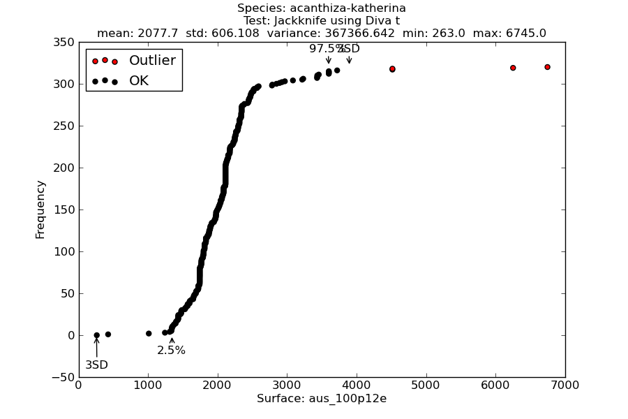 Figure 2 is an example of the a cumulative frequency curve used by this and other methods, e.g. Bioclim Classic. The figure plots occurrences against a climate variable, in this case annual precipitation. The detected outliers are shown in red. Also indicated are the 95 inter-percentile range, as well as values three standard deviation from the mean (may be missing where outside minimum and maximum sample values).
Figure 3
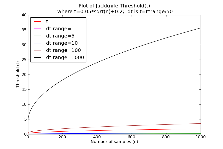 Figure 3 shows example in determining the jackknife threshold (t) using the original expression and as used in the Diva application with different ranges.
Logic
- Obtain all occurrence records for a species.
- Discard duplicate records from the sample. Methods to determine duplicates are still being refined. In this case, we should at least remove identical coordinates, and ensure there is only one occurrence for each surface grid cell. For the substrate-terrain test only include occurrences with a fine spatial precision, and that are not generalized.
- For each sub-test (i.e. set of surfaces) run the species occurrence sample through the Jackknife algorithm. Flag records that are out-of-bounds.
- Compute and save outlier metrics for each sub-test via rule-set conditions.
- Compute and save aggregated metrics via rule-set conditions.
- Compile and save histograms and statistical summary tables.
- Apply outlier metrics of selected sample records to the appropriate discarded occurrence records.
ALA Implementation
This algorithm is implemented in the Atlas of Living Australia BioCache using these five climate surfaces: BIO15 Precipitation Seasonality (Coefficient of Variation); BIO17 Precipitation of Driest Quarter; BIO23 Radiation Seasonality (Coefficient of Variation); BIO26 Radiation of the Warmest Quarter and BIO32 Mean Moisture Index of Highest Quarter MI. The test is conducted where there are 20 or more unique locations. A fail-safe is implemented so that outliers are not indicated for a surfaces where the algorithm malfunctions. This can occur where data are not continuous, or have a constrained value range.
Further comments on the algorithm are available [here] (https://github.com/AtlasOfLivingAustralia/ala-dataquality/wiki/DETECTED_OUTLIER_JACKKNIFE).
A broad discussion on spatial outlier detection methods is available here.
Some specific notes on detecting geographic outliers are available here.
Contributors
Simon Bennett, Arthur Chapman, John Tann, Jeff Tranter, Dave Martin, Lee Belbin