Jupyter ER Contents - 52North/testbed16-jupyter-notebooks GitHub Wiki
52°North targeted the implementation of three Jupyter Notebooks which combined form a single use cases. The split into sub-processes was motivated by the fact that certain steps can be parallelized (e.g. satellite scene pre-processing). This section describes the use cases, the implementation, the orchestration of the Notebooks as well as their publication on ADES instances, making them available as OGC API Processes.
The mapping of water masks in flooding situations (e.g. for river gauges affected by severe weather events) is a valuable application of Sentinel-1 SAR data. Emergency response is highly interested in the intensity and duration of floods to address flood-related damage events. In addition, the flooding history needs to be documented so that detailed information about the occurrence, frequency and duration of flooding events for the affected areas is available. This information can be used, for example, to validate flood risk assessments and planning.
The overall process is divided into three individual steps, all represented by a dedicated notebook:
-
The discovery of relevant S1 scenes (based on time and area of interest). The scenes must all cover the same area of interest and cover different points in time of a severe weather event (before, during, after)
-
The binary classification of S1 scenes (no water vs. water)
-
an aggregation of all scenes into one GeoTIFF with the count of water occurrences by pixel
The first Notebook is responsible for discovery and download of the relevant Sentinel-1 scenes. Two inputs are required:
-
area of interest (as WKT)
-
start and end date of interest (as ISO8601 date-time)
The Notebook creates a sole output:
-
array of Sentintel-1 product identifiers
The Notebook code is available at https://github.com/52North/testbed16-jupyter-notebooks/blob/master/workflow_water_masks/nb1_request/nb1.ipynb
The second Notebook is responsible for doing the image classification using the Sentinel-1 backscatter values. The implementation is based on "snappy" which is the Python library of the ESA SNAP toolbox. It takes up the outputs of Notebook #1 and applies. In particular, this process step only uses one entry of the output array. Thus, in an orchestrated workflow this Notebooks will be executed multiple times in parallel respectively for each entry of the Sentintel-1 product identifiers.
The individual steps of this notebook are describes in the following. The first aspect is the pre-processing using "snappy". It includes the application of the Orbit files, radiometric calibration, subsetting to the area of interest as well as Speckle filtering and terrain correction. An example of an intermediate result after the pre-processing is illustrated in Figure x.
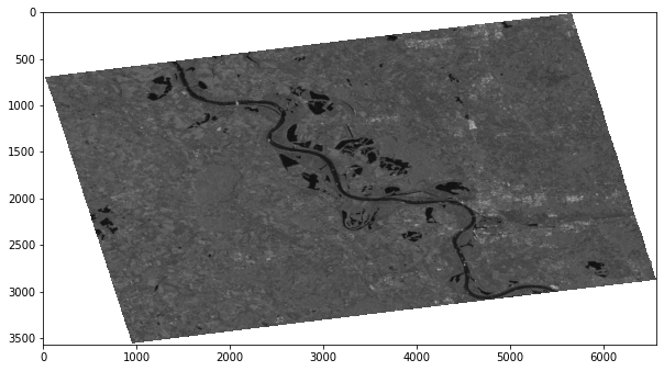
Figure x - Pre-processing result
Finally, the water pixel classification is applied: using "Multi-Otsu Thresholding", a threshold backscatter value is identified which is used to separate pixels between "water" and "no water". Figure x illustrated the identification of a threshold.
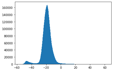
Figure x - Threshold identification
The Notebook creates a sole output:
-
a GeoTIFF representing water areas using boolean values (0 = no water, 1 = water)
An example is presented in Figure x.
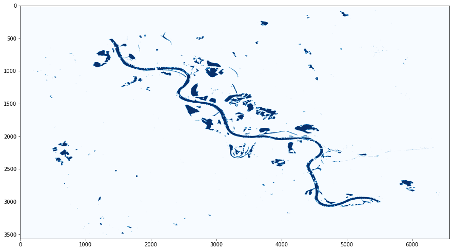
Figure x - Water pixels after Threshold application
The Notebook code is available at https://github.com/52North/testbed16-jupyter-notebooks/blob/master/workflow_water_masks/nb2_download_classify/nb2.ipynb
The last Notebook is responsible for the combination of the outputs of the previously parallelized water pixel classification. Therefore, it uses the GeoTIFFs created by Notebook #2 as the input. The algorithm counts the amount of pixels that represent water and applies a normalization to 0..1 afterwards. As the scenes are all covering the same area and are distributed over time (covering the severe weather event), the total count of pixels provides insights into flooded areas. Figure x illustrates an exemplary output.
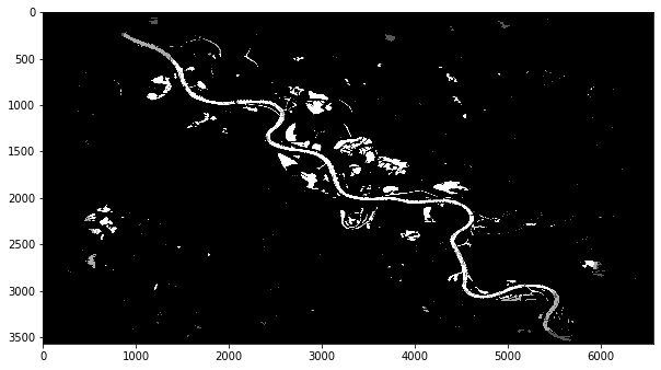
Figure x - Water Mask using Pixel Aggregation
The overall result of this process is a raster image that allows the detection of flooded areas based on the different pixel values:
-
x >= 0.9value pixels -→ persistent water body -
0.1 < x < 0.9value pixels -→ candidate for a flooded area
The Notebook creates a sole output:
-
array of Sentintel-1 product identifiers
The Notebook code is available at https://github.com/52North/testbed16-jupyter-notebooks/blob/master/workflow_water_masks/nb3_aggregate/nb3.ipynb
The chaining of the Notebooks has been established using the following technologies:
-
Papermill to externally parameterize Notebooks
-
Scrapbook to extract outputs from an executed Notebooks
-
CWL (i.e. cwl-runner) for the execution of the workflow, including input and output transfer
The CWL definition that has been developed for the orchestration of the three Notebooks is presented in Listing x.
Listing x: CWL for the Full Notebook Orchestration
#!/usr/bin/env cwl-runner
cwlVersion: v1.0
class: Workflow
inputs:
  nb1_input_notebook: File
  nb1_output_notebook: string
  nb2_input_notebook: File
  nb2_output_notebook: string
  nb3_input_notebook: File
  nb3_output_notebook: string
  parameters: File

outputs:
  nb1_output_notebook:
    type: File
    streamable: false
    outputSource: nb1_execute/output_0
  nb1_output:
    type:
      type: array
      items: string
    streamable: false
    outputSource: nb1_parse/files

  nb2_output_notebooks:
    type:
      type: array
      items: File
    streamable: false
    outputSource: nb2_execute/output_notebook
  nb2_output_results:
    type:
      type: array
      items: File
    streamable: false
    outputSource: nb2_execute/floodmask

  nb3_output_notebook:
    type: File
    streamable: false
    outputSource: nb3_execute/output_notebook
  nb3_aggregated_floodmask:
    type: File
    streamable: false
    outputSource: nb3_execute/floodmask

requirements:
  SubworkflowFeatureRequirement: {}
  ScatterFeatureRequirement: {}

steps:
  nb1_execute:
    run: nb1_request/nb1.cwl
    in:
      nb1_input_notebook: nb1_input_notebook
      nb1_output_notebook: nb1_output_notebook
      parameters: parameters
    out: [output_0]

  nb1_parse:
    in:
      input_nb: nb1_execute/output_0
    out: [files]
    run:
      class: CommandLineTool
      baseCommand: ["python3", "parse.py"]
      requirements:
        InlineJavascriptRequirement: {}
        InitialWorkDirRequirement:
          listing:
            - entryname: parse.py
              entry: |
                import scrapbook as sb
                nb = sb.read_notebook("$(inputs.input_nb.path)")
                print(','.join(list(nb.scrap_dataframe["data"])[0]))

      stdout: message

      inputs:
        input_nb:
          type: File

      outputs:
        files:
          type:
            type: array
            items: string
          outputBinding:
            glob: message
            loadContents: true
            outputEval: $(self[0].contents.replace('\n','').split(','))

  nb2_execute:
    run: nb2_download_classify/nb2.cwl
    scatter: parameters
    in:
      nb2_input_notebook: nb2_input_notebook
      nb2_output_notebook: nb2_output_notebook
      parameters: nb1_parse/files
    out: [output_notebook, floodmask]

  nb3_execute:
    run: nb3_aggregate/nb3.cwl
    in:
      nb3_input_notebook: nb3_input_notebook
      nb3_output_notebook: nb3_output_notebook
      floodmasks_geotiff: nb2_execute/floodmask
out: [output_notebook, floodmask]The ADES implementations of the other participants support the execution of CWL definitions. The integration therefore is straightforward. In addition to the above presented CWL defintion, each Notebook was accompanied with an individual CWL definition, making the Notebook integratable individually. An example CWL for Notebook #1 is presented in Listing x.
Listing x: CWL for Notebook step #1
#!/usr/bin/env cwl-runner
cwlVersion: v1.0
class: CommandLineTool
baseCommand: papermill

hints:
  DockerRequirement:
    dockerPull: workflow_water_masks_nb1request:latest

inputs:
  nb1_input_notebook:
    type: File
    inputBinding:
      position: 1
  nb1_output_notebook:
    default: output.ipynb
    type: string
    inputBinding:
      position: 2
      separate: true
      shellQuote: true
    streamable: false
  parameters:
    type: File
    inputBinding:
      position: 3
      prefix: -f

outputs:
  output_0:
    outputBinding:
      glob: $(inputs.nb1_output_notebook)
    streamable: false
    type: File