The Computer Graphics Pipeline ‐ Aidan Levy - 180D-FW-2024/Knowledge-Base-Wiki GitHub Wiki
The Computer Graphics Pipeline
Written by Aidan Levy
Extended by Marshall S. Bennett
Word Count: 3072
Overview
Computer graphics is the technology behind generating any sort of image, 2d or 3d, on a computer screen. It is both one of the most researched and optimized areas of modern desktop computers, as well as one of the most computationally heavy tasks a modern computer has to tackle. The 3d computer graphics pipeline is the process in which a list of models, information about their appearance, and the position are used to generate a 2d image to be displayed as pixels on a computer screen. This graphics pipeline is the main role of a graphics card (GPU) on a desktop computer, though most modern CPUs have simpler integrated graphics cards. The process boils down to a series of up to millions matrix multiplications once every few milliseconds, a task for which GPUs contain up to the high thousands of cores to perform in parallel.
The Pipeline
The computer graphics pipeline is specifically a series of linear transformations that transforms 3d models through different “spaces.” A space is a specific way of interpreting the coordinates so that it has significance to the task at hand. Below is an image showing a simplified model of the 3d graphics pipeline in terms of the different spaces that it changes through. Each transformation and space will be explained in the following sections.
Affine Transformations
For the sake of easy computation, a necessary goal for the following transformation is that they need to be linear and have only constant values in the transformation matrix. This means that any transformation can be computed using simple constant matrix multiplication hardware. However, this leads to a problem. It is impossible to translate any point in 3d space (meaning to slide a model in a direction without changing its shape or rotation) using only 3d linear transformation, as the origin always stays in place in any linear transformation. The solution to this is to use affine transformations and points.
The first change to make is to switch from a 3d representation to a 4d version for all points and vectors. The fourth dimension will be a constant one for points, and zero for vectors. Only the first three dimensions are actually considered, and so the fourth dimension has no physical significance to a single point. It is simply a one appended on to the end of a 3d point.
This change, however, allows us to use 4d linear transformation matrices. The idea is to use the top-left 3x3 matrix as a usual transformation matrix, and use the top-right 3 to allow for translation. An example and mathematical equation is given below.
As can be seen, the use of a 4d space with a “fake” extra point allows for the use of 4d linear transformations that allow for what appears to be a translation in 3d space, ignoring the 4th dimension.
Models and Model Space
The starting point for any 3d graphics scene is a model. Models are digital representations of a physical object. Below is an image that shows a 3d model of a rabbit at different levels of complexity.
For the purposes of 3d graphics, models are always stored as an array of vertices making up triangles. Each vertex is stored as a 4d point, with three floating point values for each real dimension and a constant 1 for the fourth dimension. Vertexes are stored in groups of threes, which together each make a small 3d triangular surface. Triangles are used for their simplicity, as there is no way to make a self-intersecting triangle and it is possible to define a direction of a triangular face if the vertices are always written in counter-clockwise order.
The starting point of the pipeline is in model space. Model space is the space in which any model is defined, and it has no correlation with the size and position of the model in the final scene. For example, a square could be defined with corners at (0,0,0) and (1,1,1). The square would be a list of 12 total triangles, two to a side. Equivalently, it would also be defined with corners at (-1,-1,-1) and (1,1,1) or any other two points in this arbitrary model space. Only the relative placement of the triangles, making the model a square, is important in this case. Model space coordinates are just the output of whatever tool the designer used to make the model. The first step in the pipeline will be to place the model into where the CPU has recorded its position. This will be a combination of translating, rotating, and scaling the model into where it belongs in the actual world of the scene
World Space
World space is the digital “world” of the scene that is being portrayed. Models are transformed from model space by an affine linear transformation that scales the model to the correct size and places and rotates it exactly how the designer likes. This is necessary to have a scene in which multiple models are arranged relative to each other. The following example transformations are common:
Through a combination of these and similar translations, a model can be placed in world space.
Eye Space
Eye space is that same world previously mentioned, except moved so that it is experienced from the viewpoint of a “camera,” which is the name for the position from which the viewer can view the world. The idea of this space is simple: instead of moving the camera around and trying to view the world from different positions and angles, simply translate the entire world so that the camera thinks that it is facing forwards at the origin, and that the world is simply in front of it like it should be. Transforming from world space to eye space is a simple combination of translating and rotating the world to place the camera at the origin. This uses the same sample matrices shown in the previous section.
Perspective Space
The next step in the pipeline is to transform the world into a perspective view. Perspective is a simple consequence of a real 3d world, and needs to be replicated in any simulated 3d world. Perspective happens because light comes in from a wide cone into a single point in a person’s eye. Thus, it can be replicated by using a transformation to distort the simulated world from a perfectly square grid into what is called a “frustum,” or a truncated pyramid. The frustum is a shape chosen because the image will be projected onto a rectangular screen. The following image shows a frustum.
The following transformation is a perspective transformation that can be used to achieve perspective in computer graphics
f and n are constants defining the size of the frustum, and S = cot(field of view angle) is the angle of the frustum.
Screen Space and Culling
The next step in the pipeline revolves around removing unnecessary edges and finishes with each triangle being actually drawn on the target screen. The first step is culling. This involves deleting any unnecessary triangles to save time in drawing triangles that are not visible.
The first type of culling is frustum culling, which is removing any triangle outside of the frustum, as they are considered outside of the field of view. This includes triangles behind, to the side, and even far enough away that they are not needed to be drawn. The next is backface culling, which means to remove any triangle that is facing “away” from the camera. The direction of a triangle is defined by the normal vector, or the cross product of two sides. Triangles are used in large part because they have a well defined normal when given in counter-clockwise vertex order, unlike more complicated shapes. The final is occlusion culling, which involves removing a triangle blocked by another. Approaches to this differ, but one common solution involves what is called a z-buffer. In a z-buffer, each pixel on a screen has a depth value. When one triangle draws, it updates the z-value. If a new triangle tries to draw to the same pixel, it will not draw if it has a higher z-value (meaning it exists further behind) than the previous triangle.
The next part of this step is the process of rasterization and lighting, in which triangles are filled in and colored with the correct color. ##Rasterization Rasterization is the process of “filling in” a triangle, meaning coloring in all the pixels that fall within it. As is usual, approaches differ. One simple example is the use of a “point in polygon” test such as below, which can be used on every pixel to see if it falls within a given triangle.
Lighting
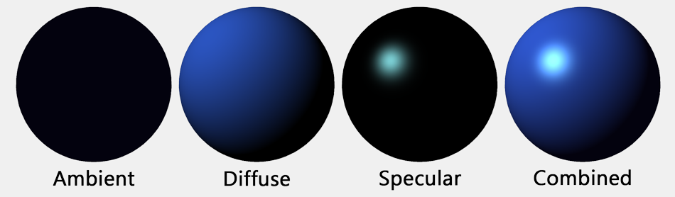
Lighting is the process of figuring out what exact color to make each pixel based off of the position and conditions of the surfaces in the scene. This process is an approximation of real-life lighting phenomenon, and has gone through many iterations. Modern lighting approximations are based on calculating different real-life lighting situations separately, and simply adding the solutions. The three components of the lighting equation are ambient lighting, diffuse lighting, and specular lighting. Isolated examples of all three are shown below.
Ambient Lighting
Ambient lighting is a small, constant amount of light added equally to all surfaces meant to simulate how light rays bouncing in a scene are able to illuminate all sides of an object. For example, even in the shadow of an object, it is still possible to see. It is calculated as a constant positive offset for every surface.
Diffuse Lighting
Diffuse lighting mimics diffuse reflection of light off of an object. This is the reflection of a matte surface like a dull plastic or paint. In the real world, this is caused by some light rays bouncing off of an object at random non-uniform angle, causing a dull color to even parts of an object not in the direct angle of the light source. It is calculated as a constant multiplied by the dot product of the normal of the surface, and the vector between each light and the surface. This means that a surface facing a light directly has greater diffuse lighting than on facing away or at an angle.
Specular Lighting
Specular lighting mimics the bright, shiny reflections on the surfaces of shiny objects like a polished metal or reflective plastic. It is caused by some light rays bouncing at a perfectly reflected angle off the material. It is modeled by reflecting the vector from the light to the surface across the normal of the triangle, then taking the dot product of that against the vector to the camera. This means that a camera being in the path of reflection from a light will see a brighter light.
Shading
The Need for Shading
As mentioned before, the preceding description of the computer graphics pipeline is missing a large and critical step towards actually drawing shapes on a screen. The above steps can transform and place a model into world space, transform it into where it should be on the screen, remove unnecessary edges, and even figure out the colors that a vertex should be. What is missing, however, is the details of how to figure out exactly what color a pixel should be based on where in the shape it is.
Flat Shading
Flat Shading is the simplest solution to this question. As can be seen in the sample image below, flat shading requires that the color be computed once for each face of a shape. Then, the entire face will be filled with that same color.
This solution leaves a lot to be desired. The key issue here is in the sharp contrast between adjacent faces. The geometric pattern of faces in a shape is obvious to the viewer, which makes the shape seem unrealistic and low quality.
Above is an example showing flat shading vs Gouraud and Phong shading, two common alternatives. While the model is the same low-quality sphere, the other shading models make the sphere seem much smoother and more realistic. Another problem with flat shading that is apparent is the fact that with larger faces and less precise color calculations, smaller details like the specular highlight get averaged out among the nearby large faces and the detail disappears.
Phong Shading
Phong shading is one of the most common shading techniques, used for simplicity and speed relative to other comparable techniques. The central idea behind Phong shading is to calculate the color of each pixel of the screen one after another. Importantly, this means that the shader needs to know the normal vector of the shape at each pixel, while we are only able to directly calculate it once per shape. Using Phong shading with the same normal value being used statically across each face leads to the same result as flat shading. In Phong shading, however, that normal value is actually calculated at each vertex and then linearly interpolated across each face, leading to a smooth transition in normal values across face. This is the key insight that allows for Phong shading to lead to a much smoother, realistic looking image.
Gouraud Shading
Gouraud shading is a very similar shading technique to Phong shading. The key difference is that in Gouraud shading, the colors are calculated using the above lighting calculations at each vertex, and then the colors themselves are interpolated across each face. This leads to a faster computation as the lighting equations don’t need to be run on every pixel. It does, however, lead to some issues. For example, specular lighting highlights like the one in the previous comparison image are just calculated at the vertex and then linearly interpolated, leading to a smoother edge on the highlight than would be present in reality.
Machine Learning in Graphics
The role of machine learning (ML) in computer graphics has been expanding rapidly, transforming traditional rendering techniques by improving performance and visual fidelity. In recent years, AI-driven solutions such as NVIDIA’s Deep Learning Super Sampling (DLSS), AMD’s FidelityFX Super Resolution (FSR), and AI-assisted texture upscaling have significantly altered the landscape of real-time rendering. These technologies leverage deep learning models to reconstruct high-resolution images from lower-resolution inputs, offering significant performance boosts while maintaining or even enhancing visual quality.
NVIDIA DLSS: AI-Powered Super Sampling
NVIDIA DLSS (Deep Learning Super Sampling) is a neural network-based upscaling technology designed to improve frame rates without sacrificing image quality. First introduced with NVIDIA’s RTX graphics cards, DLSS utilizes dedicated AI processors, called Tensor Cores, to predict and generate high-resolution images based on a low-resolution render. DLSS works by training a convolutional neural network on a vast dataset of high-quality images and their corresponding low-resolution counterparts. This allows the model to learn patterns and details that help reconstruct finer elements when upscaling lower-resolution inputs. Unlike traditional upscaling methods, which rely on basic interpolation techniques, DLSS uses temporal and spatial data from previous frames to produce sharper and more accurate visuals while reducing aliasing and artifacts. Over multiple iterations, DLSS has improved significantly. Early versions introduced some blurriness and artifacts, but newer iterations like DLSS 3 incorporate frame generation, which not only upscales images but also predicts entirely new frames using AI, effectively doubling frame rates in certain scenarios. This makes it an essential technology for demanding applications such as high-frame-rate gaming and real-time rendering in virtual reality (VR).
AMD FSR: Open-Source AI Upscaling
AMD’s FidelityFX Super Resolution (FSR) is a competing upscaling technology that aims to boost performance while maintaining image clarity. Unlike DLSS, which requires dedicated AI hardware, FSR is designed to work across a wide range of GPUs, including older and non-RTX cards, by relying on a combination of spatial upscaling and sharpening algorithms. FSR 1.0, the first iteration, used a spatial upscaling technique that applied contrast-adaptive sharpening to enhance details after upscaling a lower-resolution render. While effective, it lacked the temporal stability of DLSS. FSR 2.0 and later versions improved upon this by incorporating temporal anti-aliasing (TAA), allowing for better detail reconstruction and reduced ghosting artifacts.FSR has gained popularity due to its open-source nature and cross-platform compatibility. It enables developers to implement upscaling solutions without requiring proprietary hardware, making it a widely accessible alternative to DLSS.
AI-Assisted Texture Upscaling
Another significant application of machine learning in graphics is AI-assisted texture upscaling. Traditional methods of enhancing texture resolution, such as bicubic interpolation, often produce blurry or pixelated results when increasing the size of low-resolution textures. AI-driven upscaling, however, leverages deep learning models trained on high-quality textures to infer missing details and enhance textures with remarkable clarity.Techniques such as ESRGAN (Enhanced Super-Resolution Generative Adversarial Network) have been widely adopted for texture enhancement in both modern and retro gaming. This allows older games to receive high-resolution texture packs without requiring artists to manually recreate assets. AI-assisted texture upscaling is also used in real-time applications, where lower-resolution textures can be dynamically enhanced to save memory bandwidth while maintaining high visual fidelity.
The Future of AI in Graphics
Machine learning’s role in graphics is poised to grow even further. Future developments could bring more efficient real-time rendering techniques, improved denoising for ray tracing, and even AI-generated assets that reduce development time for game designers. As AI models become more sophisticated and hardware continues to evolve, AI-driven graphics enhancements will likely play a central role in achieving photorealistic rendering with minimal computational overhead. By integrating AI into the graphics pipeline, developers can push the boundaries of real-time rendering, making high-quality visuals accessible even on lower-end hardware. With technologies like DLSS, FSR, and AI-assisted upscaling leading the charge, the future of computer graphics is set to be faster, more efficient, and visually stunning.
Sources
https://graphicscompendium.com/intro/
https://medium.com/@rakadian/graphics-pipeline-9e4bb2d28f58
https://stanford.edu/class/ee267/lectures/lecture2.pdf
https://www.khronos.org/opengl/wiki/Rendering_Pipeline_Overview
https://www.thecandidstartup.org/2023/03/13/trip-graphics-pipeline.html
https://www.mauriciopoppe.com/images/flat-shading.svg
https://i.pcmag.com/imagery/encyclopedia-terms/flat-shading-_shading.fit_lim.size_1050x.gif
https://clara.io/img/pub/amb_diff_spec.png
https://www.nvidia.com/en-us/geforce/technologies/dlss/
https://www.amd.com/en/products/graphics/technologies/fidelityfx/super-resolution.html