Main control structures for energy systems - guidosassaroli/controlbasics GitHub Wiki
This section presents some of the major control structures for energy systems, remaining in the Linear Time-Invariant (LTI) context.
Feedforward Compensation
The objective of this technique is to reduce the influence on the controlled variable y(t) of a measurable disturbance d(t) acting on the loop forward path. This can be achieved by computing K(s) so that Y(s)/D(s) is ideally zero.
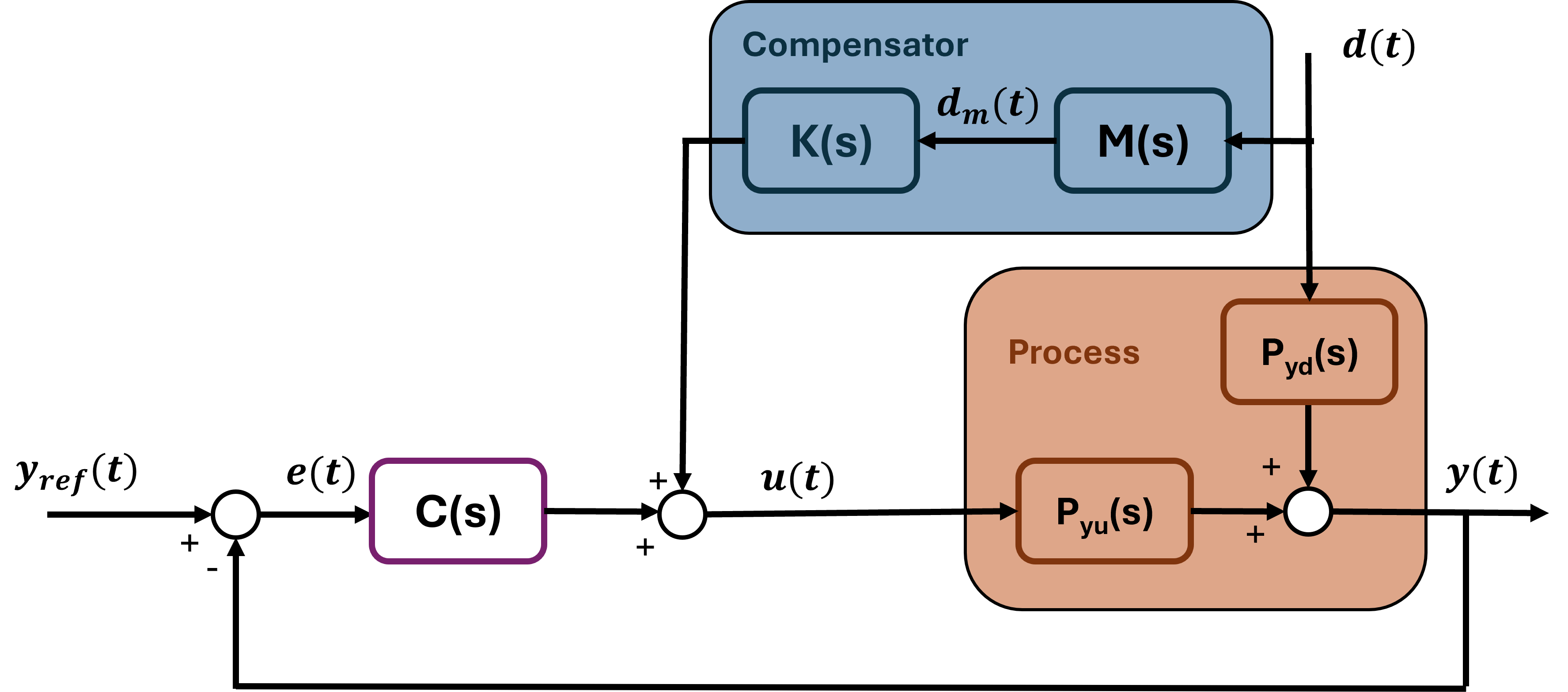
$$ \frac{P_{yd}(s)+M(s)K(s)P_{yu(s)}}{1+R(s)P(s)} = 0 $$ Then, in order to get this the ideal compensator is: $$ K_{ID}(s) = - \frac{P_{yd}(s)}{M(s)P_{yu}(s)} $$
This compensator is ideal because it has more zeros than poles, and poles in the right-half plane (causing critical cancellations). The real compensator is typically derived by omitting some zeros and/or adding poles. This compensation is valid only up to a certain frequency, because at high frequencies K(jω) starts to differ from K_ID(jω).
Cascade Control
Cascade control combines two feedback loops: the output of one controller (the primary) adjusts the set-point of a second controller (the secondary). It is used to reduce the effect of an immeasurable disturbance d_I(t) that affects some measurable intermediate variable y_I(t).
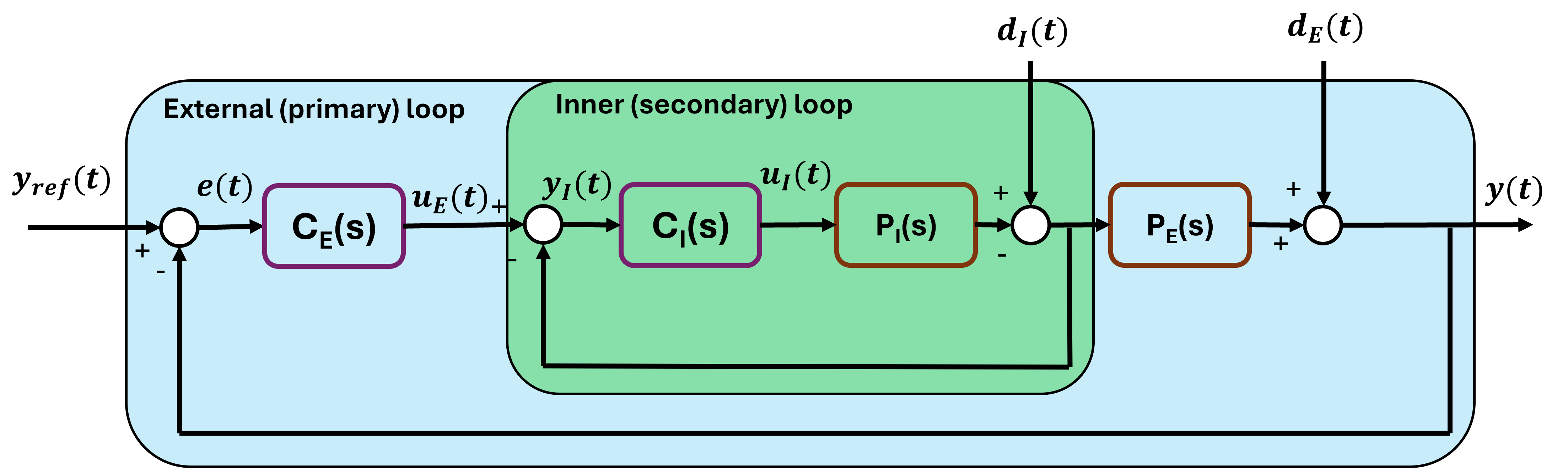
The inner (secondary) loop must be fast enough to hide both the dynamics of P_I and the effects of d_I from the outer (primary) loop.
Smith Predictor
The Smith Predictor is used when the process delay is large. It allows improved performance without sacrificing stability.
It uses an internal model to predict the delay-free response ŷ(t) of the process. It compares this prediction ŷ(t) with the desired setpoint y_ref(t) to determine the control action u.
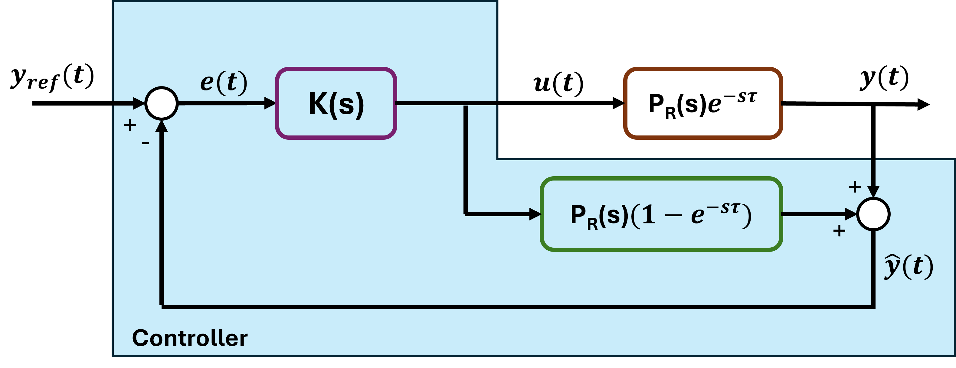
In the scheme we can see that: $$ \frac{\hat{Y}(s)}{U(s)} = P_R(s) $$
where P_R(s) is assumed rational.
Requirements:
- A model
P_R(s)of the process dynamics and an estimateτof the process dead time. - Adequate settings for the compensator dynamics
K(s).
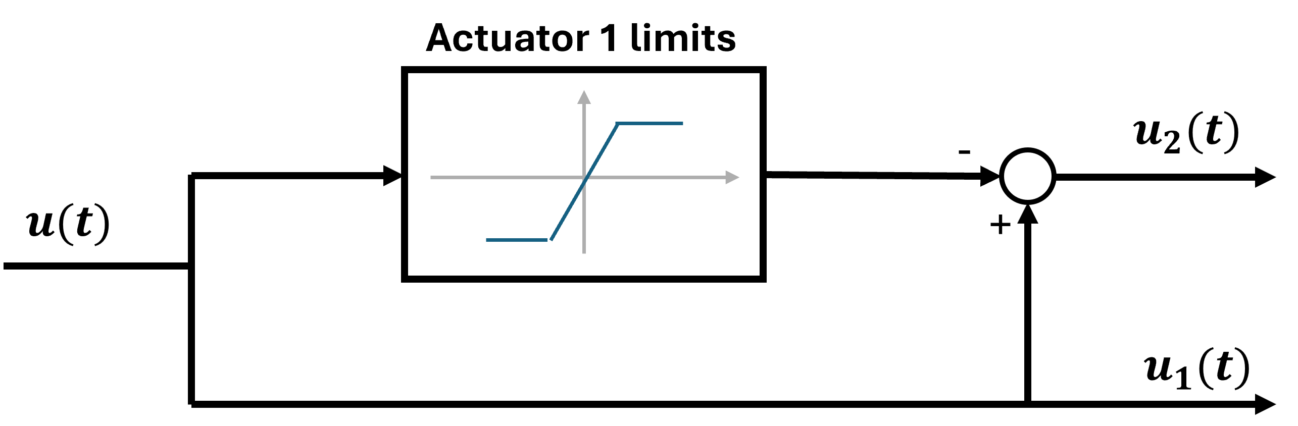
Split Range
The purpose of this actuation control scheme is to make two actuators behave like a single one by having each of them act in a different range of control variable. A typical example is a temperature controller with one actuator for heating and one for cooling. This is easily achieved splitting the output into two different areas, one for the first actuator ($u_1 \in [0,1]$) and one for the second actuator ($u_2 \in [-1,0]$). The control action is defined in the following domain: $u \in [-1,1]$. The simple setting is the following: \newline
$$
u_1 =
\begin{cases}
u & u \geq 0\
0 & u < 0
\end{cases}
$$
$$
u_2 =
\begin{cases}
0 & u \geq 0\
-u & u < 0
\end{cases}
$$
Remark: A dead zone may be added around u = 0 to avoid frequent switching between actuators.
Daisy-Chaining
The purpose of this technique is to have several actuators activated in sequence when the previous one has reached its maximum. This logic is to start with the most energy-efficient actuator and the less efficient actuators intervene only if its necessary.
This scheme can be easily generalized to an arbitrary number of actuators.
Hint: Sometimes a dead zone is introduced around the transition to avoid switching in and out the two actuators too frequently.