Table of Contents Objective Activates & Tasks Progress & Notes Conclusion, Outlook, & Discussion References

The objective goal of this project is to continue with gene analysis while also incorporating gene network mapping and interactions. This means that the goal of this assignment is to rank genes based on differential expression using the normalized expression data generated in Assignment #1. Perform thresholded over-representation analysis (ORA) on the ranked list in Assignment #2 to reveal dominant genes/themes in the top set of genes. Using this data, attempt to figure out if there is a relationship between the genes and the diseases that they produce. Then check whether we can get the same, if not identical, results using non-threshold analysis, which would lead us to believe that there are genes responsible for the impacts of the impacted groups. We are more focused on the pathways that are being represented and their network interactions, so that is why we will be using Cytoscape + Enrichment Map to visualize our outputs.

Here is the link to the page with the tasks and outlines for this assignment.

The procedure and general skeletal structure for this assignment are as follows:

1. Use non-thresholded analysis to determine pathways and genes of interest
2. This will lead them to be sorted by rank
3. Sort genes by order by their most positive to most negative enrichment ranks.
4. Extrapolate ideas and data from this enrichment data and compare them to assignment 2
5. Visualize the map interactions on Cytoscape.
6. Interpret results and find links to other datasets.

Here is the link to the dataset for this assignment that the analysis was performed on; GSE193417, with the accompanying paper titled Lower Levels of GABAergic Function Markers in Corticotropin-Releasing Hormone-Expressing Neurons in the sgACC of Human Subjects With Depression of which can be found here at this link on here and its respective DOI: 10.1016/j.jbc.2022.101652.

I decided to make all the important information to be easily accessible in terms of code and data objects, saved the necessary files, in a common directory so that in the case that I need to make changes or do something differently I do not have to go through multiple files to make the changes. While I understand that this separation and depending on other notebooks as a child, is important, there isn't enough code here for me to really justify separating it up. Maybe if each component of the analysis was extremely meticulous and I had done the best fit model for each individual data type or had done things that would take up an exorbitant amount of time, but in cases like this where everything is already set up, it's just significantly easier. In this case, it turned out to be a lot more of a benefit than a hindrance as a lot of the lecture code did not really work as well as I had wanted it to, even when I used the proper image from docker. I still do not know why, this is the case, but in any case, I had to use the command line, or find alternative methods for the same steps.

So, with the ordered gene list from assignment 2, I was able to calculate the ranks based on the formulae given in the lecture notes and from the Baderlab gene analysis walkthrough. There were different variations on what you could multiply, like the tvalue*logFC but otherwise, you'd get some sort of ranking that is feasible to use in the next steps.

Learning GESA application and how to get the correct files was slightly more difficult, but eventually, I figured out how and what to do base on relating it to the lecture notes, using the .rnk file of the genes we created in R was the first step, and then using the pre-ranked option to generate all the interactions and files for the dataset eventually led me to get a pre-ranked output file. I have this on my computer but I wasn't able to upload it to GitHub, I can upload it to other file-sharing websites but the edb output file in the directory should be found in the files tab for my wiki. In it, was GESA's own rnk file, a gene sets file, etc which can be used on profiler if need be to get more data and analysis for genes. What to note here is that we could have used this instead of doing assignment 1 and assignment 2, because we have the option of doing the analysis and running the genes through the GESA to get a normalized, cleaned and mapped dataset. The reason why we didn't do it this way, is probably because to appreciate the applications and tools that have already been established, also r studio is significantly faster as I have noticed, that most of the software we used is very limited to the computer's specs.

We then made network maps, and visualize it using cytoscape using the na_pos and na_neg, .rnk file, and the .gmt file for mapping the pathways. This will tell us what pathways and what genes are mostly related in this dataset. This part was quite difficult for me, as I could not get the data to play well. It was extremely weird that when I would set the FDR value to 0.01, I would get 0 hits. I am not sure why this was the case at all. So, I left my FDR rate at .9, now I know this is really not the correct way to do this, but without it, I would not have had anything at all to visualize, and analyze. This gave me 371 nodes, with coincides with the number of total hits from the GESA analysis we had earlier. Both of these are noted in the journal. To get the information to load incorrectly, I had to use the CLI arguments, to select the files and commands. This was the only way that I was able to load the data and generate network maps. However, after I had the initialized data set loaded in, I was able to make the maps, annotate them etc. With relative ease.

Lastly came the analysis, and interpretation portion of the assignment, which essentially reiterated the fact that there were some gene interactions, and their causation. Since this was a non-thresholded gene analysis, we did not cross off values or genes arbitrarily, and it was mostly determined by the p values and ranks as well as their ordering of the genes based on calculated values. This order of the genes was very similar to the thresholded analysis that we did in A2.

To talk about some problems that I had, it was mostly learning how to use GSEA and Cytoscape because it was all new, and I could not see the results of my changes for a graph or a geneset until minutes later, which lead to a lot of frustration. Waiting to see my results really demotivated me into just trying new things and randomly experimenting as I usually do. In this case I meticulously researched methods and ideas before making any sudden changes to my map or gene set.

In this scenario, the relationship between individuals who suffer from MDD and those who do not is undeniably linked to genes, as the article predicted. Because genes code for everything in us, we diverge from our intended roles and behaviours if genes fail or there are regulatory discrepancies. The gprofiler outputs are a simple way of showing what types of pathways we can expect to be most affected as well as being some of the top hits, which was 100% the case when we did our GSEA non-thresholded analysis, as the pathway hits on the profiler constituted a hit across the board, as I have stated before, it is honestly amazing to me that there is such a strong relationship that has transcended all three assignments, each in their own different way, with A2 and A3 being the most interconnected because of their resulting outputs, one showing the many genes of interest, in A2s case, with A3 showing the many pathways with encompassing genes.

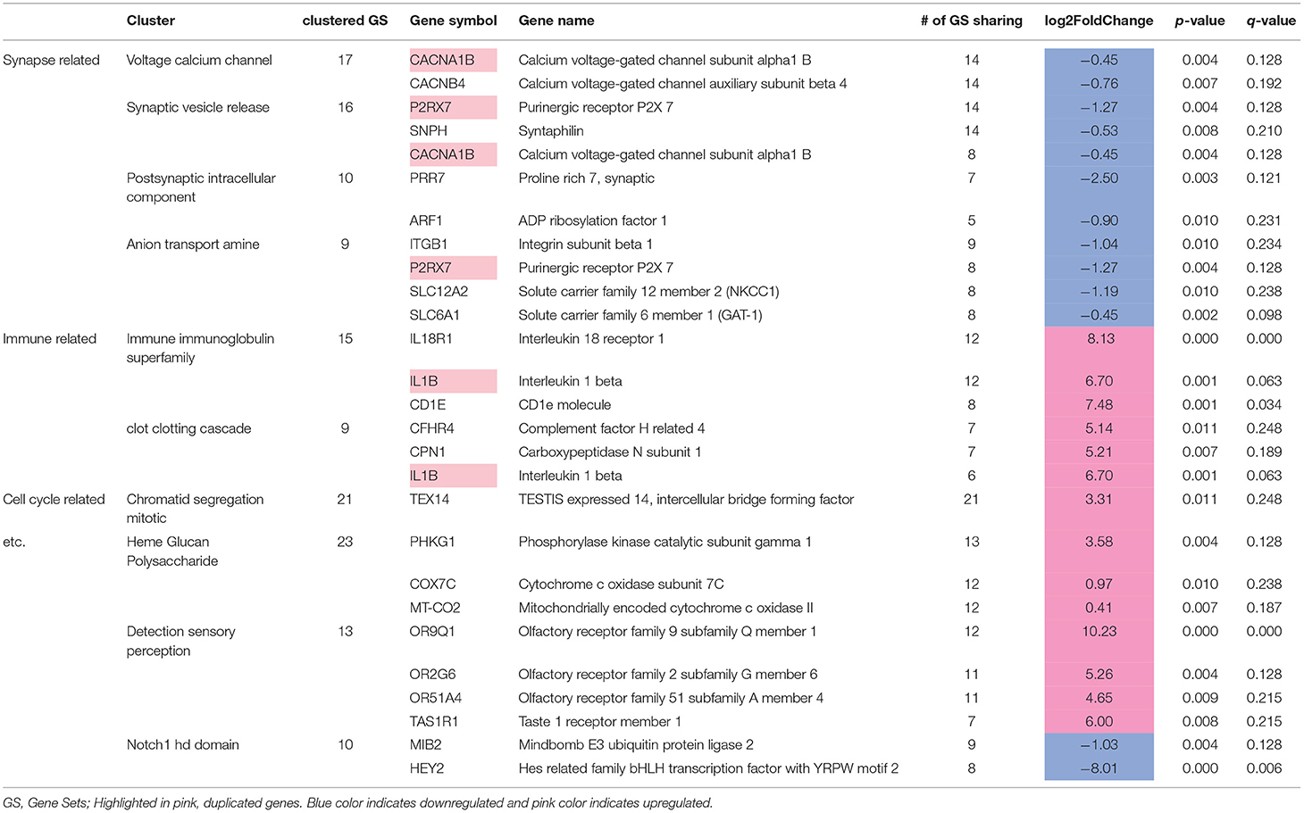
In conclusion, the idea that there was a strong correlation between the pathways and their constituents was supported in the paper. Though, it should be noted again for redundancy that we need more samples. This way any outlier data can be easily identified and normalized. In this assignment, I used the same analysis method as the authors of the paper. I got similar gene pathways and it matched up the number of genes that were also represented, based on table 5 of the paper. In closing, I would like to say that more samples would have really been interesting to see, expecially if this was more than a coincidence, as even though there are 6 samples for MDD and control, the authors themselves have mentioned that more samples could have lead to a stronger conclusion. So while more research and methods are needed, it is getting harder and harder to not say that there isn't some sort of relationship.

A side not that I wanted to make at the end was that I am very interested in redoing these assignments, using different methods; for normalization, for cleaning, and seeing if my results diff, as well as doing what the authors did to see if I can get the exact same results as them, mainly using GeneMania to map the genes etc. If I cannot get the same answers it means some of the conclusions or methods I was using are incorrect and I would be keen to know which ones work and which methods don't of it is all context dependent.

1. Bonnin, S. (2022). 19.11 Volcano plots | Introduction to R. Biocorecrg.github.io. Retrieved 13 April 2022, from https://biocorecrg.github.io/CRG_RIntroduction/volcano-plots.html.

2. Cotter, D., Mackay, D., Landau, S., Kerwin, R., & Everall, I. (2001). Reduced Glial Cell Density and Neuronal Size in the Anterior Cingulate Cortex in Major Depressive Disorder. Archives Of General Psychiatry, 58(6), 545. https://doi.org/10.1001/archpsyc.58.6.545

3. Differential Expression with Limma-Voom. Ucdavis-bioinformatics-training.github.io. (2022). Retrieved 13 April 2022, from https://ucdavis-bioinformatics-training.github.io/2018-June-RNA-Seq-Workshop/thursday/DE.html.

4. Duan, E. (2022). R|Py notes: Volcano plots with ggplot2. R|Py notes. Retrieved 13 April 2022, from https://erikaduan.github.io/posts/2021-01-02-volcano-plots-with-ggplot2/.

5. Falcon, S., & Gentleman, R. (2006). Using GOstats to test gene lists for GO term association. Bioinformatics, 23(2), 257-258. https://doi.org/10.1093/bioinformatics/btl567

6. Geistlinger, L., Csaba, G., Santarelli, M., Ramos, M., Schiffer, L., Turaga, N., Law, C., Davis, S., Carey, V., Morgan, M., Zimmer, R., & Waldron, L. (2021). Toward a gold standard for benchmarking gene set enrichment analysis. Briefings in bioinformatics, 22(1), 545–556. https://doi.org/10.1093/bib/bbz158

7. Huang, D., Sherman, B., & Lempicki, R. (2008). Bioinformatics enrichment tools: paths toward the comprehensive functional analysis of large gene lists. Nucleic Acids Research, 37(1), 1-13. https://doi.org/10.1093/nar/gkn923

8. Lin, L., & Sibille, E. (2013). Reduced brain somatostatin in mood disorders: a common pathophysiological substrate and drug target?. Frontiers In Pharmacology, 4. https://doi.org/10.3389/fphar.2013.00110

9. Oh, H., Newton, D., Lewis, D., & Sibille, E. (2022). Lower Levels of GABAergic Function Markers in Corticotropin-Releasing Hormone-Expressing Neurons in the sgACC of Human Subjects With Depression. Frontiers In Psychiatry, 13. https://doi.org/10.3389/fpsyt.2022.827972

10. Peng, R. (2022). R Programming for Data Science. Bookdown.org. Retrieved 13 April 2022, from https://bookdown.org/rdpeng/rprogdatascience/.

11. Shelton, R., Claiborne, J., Sidoryk-Wegrzynowicz, M., Reddy, R., Aschner, M., Lewis, D., & Mirnics, K. (2010). Altered expression of genes involved in inflammation and apoptosis in frontal cortex in major depression. Molecular Psychiatry, 16(7), 751-762. https://doi.org/10.1038/mp.2010.52

12. Steipe, B., & Isserlin, R. (2022). BCB420 - Computational System Biology. Bcb420-2022.github.io. Retrieved 13 April 2022, from https://bcb420-2022.github.io/General_course_prep/index.html#attributions.

13. Steipe, B., & Isserlin, R. (2022). BCB420 - Computational System Biology. Bcb420-2022.github.io. Retrieved 13 April 2022, from https://bcb420-2022.github.io/R_basics/.

14. Steipe, B., & Isserlin, R. (2022). BCB420 - Computational System Biology. Bcb420-2022.github.io. Retrieved 13 April 2022, from https://bcb420-2022.github.io/Bioinfo_Basics/.

15. Lecture modules: https://q.utoronto.ca/courses/248455/modules

16. Uku Raudvere, Liis Kolberg, Ivan Kuzmin, Tambet Arak, Priit Adler, Hedi Peterson, Jaak Vilo: g:Profiler: a web server for functional enrichment analysis and conversions of gene lists (2019 update) Nucleic Acids Research 2019; doi:10.1093/nar/gkz369 [PDF].