In current GeoDa (version < 1.12.1.227), there is a "Aggregate" feature that allows users to aggregate or group table records that have the same values for a specified attribute (also called a "key" variable). When grouping records using this "key" variable, one can specify an aggregate function (count/average/max/min/sum) and apply it on several selected variables. This "Aggregate" function works only on table data, and the aggregated results can be saved as a table-only dataset (e.g. csv, dbf etc.)

For example, using GeoDa to aggregate the Guerry dataset by Region and compute Average values of each group on variables (Crm_prn, Donatns, Crm_prs, Crm_prp):

The results are saved in a csv file:

In GIS, the dissolve algorithm takes a polygon layer (map) and group the polygons that have the same values by merging adjacent polygons into single geometries. It is very similar to "Aggregate" function mentioned above, and the difference is that dissolve works on geometries but "Aggregate" works on table records. I think it will be useful to have a dissolve + "Aggregate" function in spatial data analysis, so that users can dissolve geometries and get new attributes that have been computationally aggregated from original dataset and attached to dissovled geometries.

In this implementation, a menu option "Dissolve" will be added under "Tools->Shape" menu in GeoDa. After click this menu item, a "Dissolve" dialog will be shown to allow users to specify a variable that defines clusters for dissolving. Other controls in this dialog will be similar with above "Aggregate" dialog: Users can select multi-variables and an aggregate function, and the aggregated results will be attached to the dissolved geometries. When saving the results, the dissolved geometries and their attributes will be saved to a new dataset, which can be loaded as a new map layer in GeoDa.

For example, the Guerry dataset (France 1830) can be grouped/aggregated by the region attribute.

Here is a "Unique Value" map of Guerry dataset using region attribute showing the spatial distributions of the regions:

One can use the "Dissolve" feature to create a new map with 5 new polygons that represent "E", "N", "C", "S", and "W" by dissolving the polygons with same region value. If none variables were specified in "Dissolve" dialog, the newly created map will only contains two fields: one is the variable selected for dissolving dept, and another is called AGG_COUNT, which shows the number of dissolved or merged polygons from original map.

Users can select variables that will be aggregated in "Dissolve" dialog, and the values will be aggregated for the newly created polygons. For example, one can create a U.S. homicide dataset at state level using "Dissolve" feature and a U.S. homicide dataset at county level (see US county homicide sample data: natregime).

"Dissolve" can also be used to create a new cluster map from clustering results, e.g. spatially constrained clustering methods: SKATER, REDCAP, or max-p.

For example, one can apply SKATER on Guerry dataset to find clusters using six variables (Crm_prs, Crm_prp, Litercy, Donatns, Infants and Suicids). The results is shown in this figure:

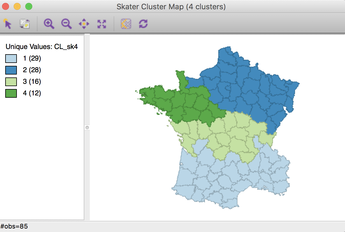
The clustering results are saved in variable CL_sk4 in the table. One can apply dissolve on this variable to create a new cluster map: