1%29 Sehender Raum %3A Seeing Space - 3a1b2c3/seeingSpace GitHub Wiki
- "Classic rendering" in computer graphics, since 1970s
- Inverse and Differential rendering (aka "Computervision")
- Neural Rendering, ca 1990s
-
Image-based rendering (IBR): Plenoptic function and capture
- The plenoptic function 8D, Gabriel Lippmann, 1908
- Static 5D and 4D Lightfields: capture and rendering (Gabriel Lippmann, 1908)
- Open problems / research topics
- Conclusion
Table of contents generated with markdown-toc
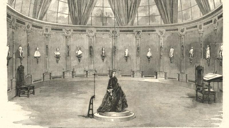
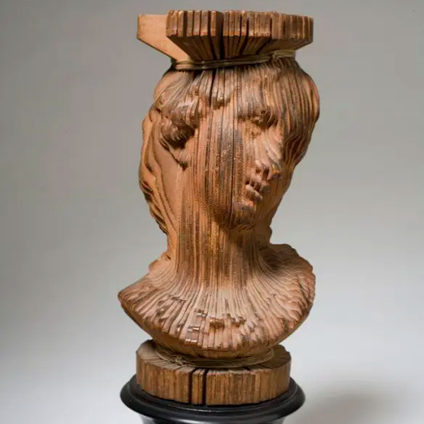
- A 1800 century analogous version of nerfs https://hackaday.com/2022/10/02/in-a-way-3d-scanning-is-over-a-century-old/
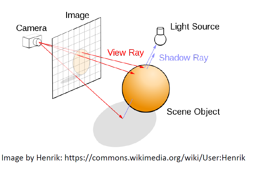
Classical computer graphics methods approximate the physical process of image formation in the real world: light sources emit photons that interact with the objects in the scene, as a function of their geometry and material properties, before being recorded by a camera. This process is known as light transport. The process of transforming a scene definition including cameras, lights, surface geometry and material into a simulated camera image is known as rendering.
The two most common approaches to rendering are rasterization and raytracing.
- Rasterization is a feedforward process in which geometry is transformed into the image domain, sometimes in back-to-front order known as painter’s algorithm.
- Raytracing is a process in which rays are cast backwards from the image pixels into a virtual scene, and reflections and refractions are simulated by recursively casting new rays from the intersections with the geometry.
The rendering equation (published in 1986)
The rendering equation describes physical light transport for a single camera or the human vision. A point in the scene is imaged by measuring the emitted and reflected light that converges on the sensor plane. Radiance (L) represents the ray strength, measuring the combined angular and spatial power densities. Radiance can be used to indicate how much of the power emitted by the light source that is reflected, transmitted or absorbed by a surface will be captured by a camera facing that surface from a specified angle of view.


Source: https://www.semanticscholar.org/paper/Inverse-Rendering-and-Relighting-From-Multiple-Plus-Liu-Do/da1ba94e01596d0241d7d426b071ae9731d148b3, https://www.mdpi.com/2072-4292/13/13/2640, Rendering for Data Driven Computational Imaging, Tristan Swedish
Inverse graphics attempts to take sensor data and infer 3D geometry, illumination, materials, and motions such that a graphics renderer could realistically reproduce the observed scene. Renderers, however, are designed to solve the forward process of image synthesis. To go in the other direction, we propose an approximate differentiable renderer (DR) that explicitly models the relationship between changes in model parameters and image observations. Differentiable rendering enables optimization of 3D object properties like the geometry of a mesh. Unlike traditional rendering, differentiable rendering can backpropagate gradients from image space to 3D geometry.
- https://github.com/weihaox/awesome-neural-rendering
- https://sites.google.com/princeton.edu/neural-optics/


Source: http://rgl.epfl.ch/publications/NimierDavidVicini2019Mitsuba2
Inverse rendering and differentiable rendering have been a topic of research for some time. However, major breakthroughs have only been made in recent years due to improved hardware and advancements in deep learning.
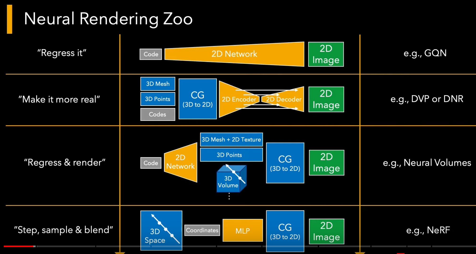
Is a relative new technique that combines classical or other 3D representation and renderer with deep neural networks that rerender the classical render into a more complete and realistic views. In contrast to Neural Image-based Rendering (N-IBR), neural rerendering does not use input views at runtime, and instead relies on the deep neural network to recover the missing details. Deepfakes are an early neural rendering technique in which a person in an existing image or video is replaced with someone else's likeness. The original approach is believed to be based on Korshunova et al (2016), which used a convolutional neural network (CNN).
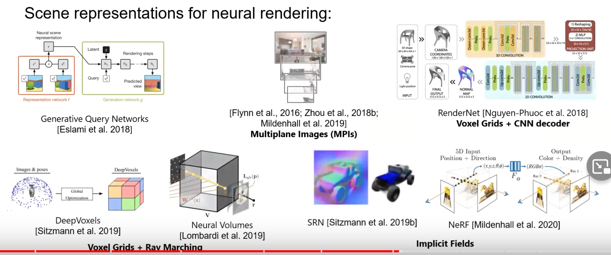
A typical neural rendering approach takes as input images corresponding to certain scene conditions (for example, viewpoint, lighting, layout, etc.), builds a "neural” scene representation from them, and "renders” this representation under novel scene properties to synthesize novel images.
The learned scene representation is not restricted by simple scene modeling approximations and can be optimized for high quality novel images. At the same time, neural rendering approaches incorporate ideas from classical graphics—in the form of input features, scene representations, and network architectures—to make the learning task easier, and the output more controllable. Neural rendering has many important use cases such as semantic photo manipulation, novel view synthesis, relighting, free viewpoint video, as well as facial and body reenactment.


Source: Advances in Neural Rendering, https://www.neuralrender.com/ Source: Advances in Neural Rendering, https://www.neuralrender.com/
Artifacts such as ghosting, blur, holes, or seams can arise due to view-dependent effects, imperfect proxy geometry or too few source images. To address these issues, N-IBR methods replace the heuristics often found in classical IBR methods with learned blending functions or corrections that take into account view-dependent effects.
Source: Advances in Neural Rendering, https://www.neuralrender.com/
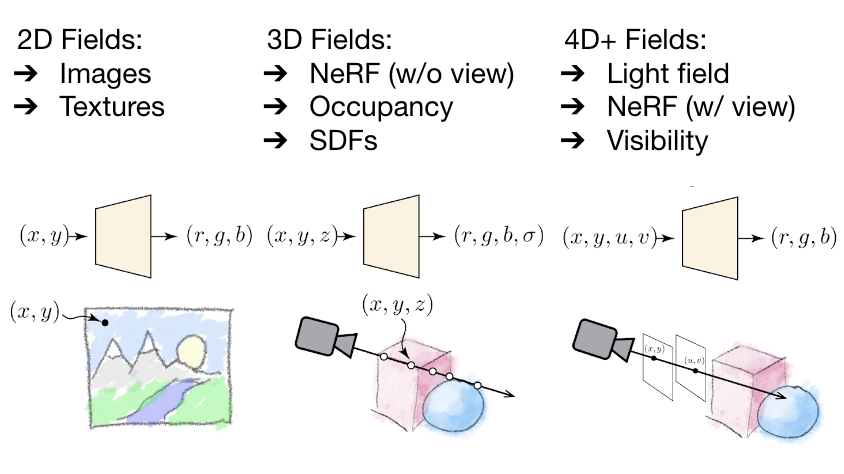
Media of any dimension can be learned by neural networks, in some cases more space efficient than with traditional storage formats.
Computational imaging (CI) is a class of imaging systems that, starting from an imperfect physical measurement and prior knowledge about the class of objects or scenes being imaged, deliver estimates of a specific object or scene presented to the imaging system.
In contrast to classical rendering, which projects 3D content to the 2D plane, image-based rendering techniques generate novel images by transforming an existing set of images, typically by warping and compositing them together. The essence of image-based rendering technology is to obtain all the visual information of the scene directly through images. Its used in computer graphics and computer vision, and it is also widely used in virtual reality technology.
The world as we see it using our eyes is a continuous three-dimensional function of the spatial coordinates. To generate photo-realistic views of a real-world scene from any viewpoint, it not only requires to understand the 3D scene geometry, but also to model complex viewpoint-dependent appearance resulting of light transport phenomena. A photograph is a two-dimensional map of the “number of photons” that map from the three-dimensional scene.
While the rendering equation is a useful model for computer graphics some problems are easier to solve by a more generalized light model.

 Source: https://en.wikipedia.org/wiki/Compound_eye, Rendering for Data Driven Computational Imaging, Tristan Swedish
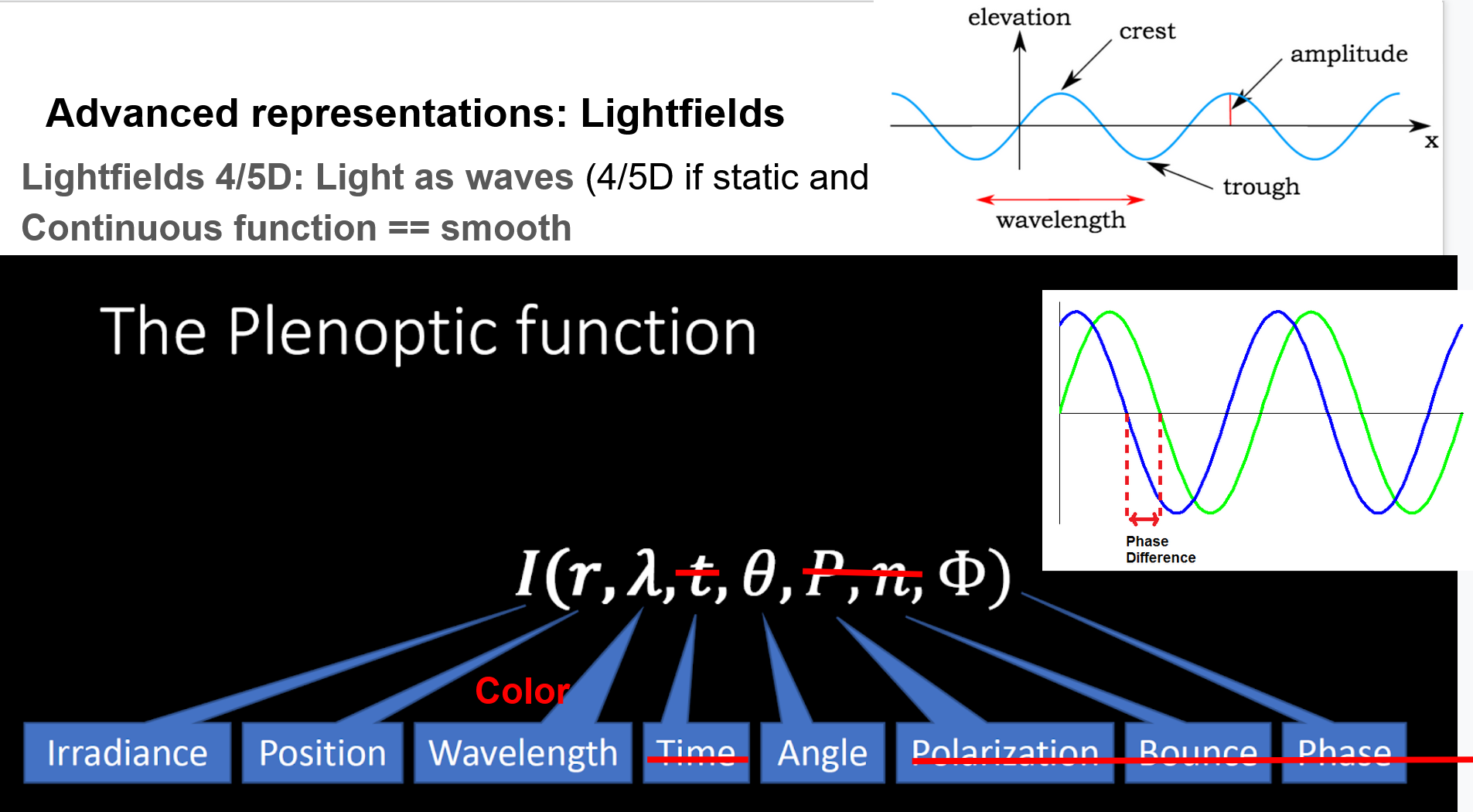
The plenoptic function describes the degrees of freedom of a light ray with the parameters: Irradiance, position, wavelength, time, angle, phase, polarization, and bounce.


Source: Rendering for Data Driven Computational Imaging, Tristan Swedish, https://www.blitznotes.org/ib/physics/waves.html, https://courses.lumenlearning.com/boundless-chemistry/chapter/the-nature-of-light/
Light has the properties of waves. Like ocean waves, light waves have crests and troughs.
- The distance between one crest and the next, which is the same as the distance between one trough and the next, is called the wavelength.
- Wave phase is the offset of a wave from a given point. When two waves cross paths, they either cancel each other out or compliment each other, depending on their phase.
- Irradiance is the amount of light energy from one thing hitting a square meter of another each second. Photons that carry this energy have wavelengths from energetic X-rays and gamma rays to visible light to the infrared and radio. The unit of irradiance is the watt per square meter.
- Polarization and Bounce are often omitted for simplicity
- The full equation is also time dependent.
Light-field capture was first proposed in 1908 by Nobel laureate physicist Gabriel Lippmann (who also contributed to early color photography). If Vx, Vy, Vz are fixed, the plenoptic function describes a panorama at fixed viewpoint (Vx, Vy, Vz). A regular image with a limited field of view can be regarded as an incomplete plenoptic sample at a fixed viewpoint. As long as we stay outside the convex hull of an object or a scene, if we fix the location of the camera on a plane, we can use two parallel planes (u,v) and (s,t) to simplify the complete 5D plenoptic function to a 4D lightfield plenoptic function.
A Light field is a mathematical function of one or more variables whose range is a set of multidimensional vectors that describe the amount of light flowing in every direction through every point in space*. It restricts the information to light outside the convex hull of the objects of interest. The 7D plenoptic function can under certain assumptions and relaxations simplify o a 4D light field, which is easier to sample and operate on. A hologram is a photographic recording of a light field, rather than an image formed by a lens. A light field is a function that describes how light transport occurs throughout a 3D volume. It describes the direction of light rays moving through every x=(x, y, z) coordinate in space and in every direction d, described either as θ and ϕ angles or a unit vector. Collectively they form a 5D feature space that describes light transport in a 3D scene.
The magnitude of each light ray is given by the radiance and the space of all possible light rays is given by the five-dimensional plenoptic function. The 4D lightfield has 2D spatial (x,y) and 2D angular (u,v) information that is captured by a plenoptic sensor.
- the incident light field Li(u, v, alpha, beta) describing the irradiance of light incident on objects in space
- the radiant light field Lr (u, v, alpha, beta) quantifying the irradiance created by an object
- time is an optional 5th dimension
Light field rendering [Levoy and Hanrahan 1996] eschews any geometric reasoning and simply samples images on a regular grid so that new views can be rendered as slices of the sampled light field. Lumigraph rendering [Gortler et al. 1996] showed that using approximate scene geometry can ameliorate artifacts due to undersampled or irregularly sampled views. The plenoptic sampling framework [Chai et al. 2000] analyzes light field rendering using signal processing techniques and shows that the Nyquist view sampling rate for light fields depends on the minimum and maximum scene depths. Furthermore, they discuss how the Nyquist view sampling rate can be lowered with more knowledge of scene geometry. Zhang and Chen [2003] extend this analysis to show how non-Lambertian and occlusion effects increase the spectral support of a light field, and also propose more general view sampling lattice patterns. Rendering algorithms based
One type uses an array of micro-lenses placed in front of an otherwise conventional image sensor to sense intensity, color, and directional information. Multi-camera arrays are another type. Compared to a traditional photo camera that only captures the intensity of the incident light, a light-field camera provides angular information for each pixel.
In principle, this additional information allows 2D images to be reconstructed at a given focal plane, and hence a depth map can be computed. While special cameras and cameras arrangements have been build to capture light fields it is also possible them with a conventional camera or smart phone under certain constraints (see Crowdsampling the Plenoptic Function).


Source: Stanford light field camera; Right: Adobe (large) lens array, source https://cs.brown.edu/courses/csci1290/labs/lab_lightfields, "Lytro Illum", a discontinued commercially available light field camera
Newer work on those kind of hardware setups by meta https://robust-dynrf.github.io/.
See also 2) Nerf (radiance fields) basics, encodings and frameworks
Source: Advances in Neural Rendering, https://www.neuralrender.com/
 * General purpose format, can store images, points, voxels, meshes, compression
* Cloudy blurry artifacts when not enough data available
* Can handle reflection and transparent objects, small details, fuzzy objects
* Not meant for survey/measuring, can generate low-res geometry via marching cubes
* General purpose format, can store images, points, voxels, meshes, compression
* Cloudy blurry artifacts when not enough data available
* Can handle reflection and transparent objects, small details, fuzzy objects
* Not meant for survey/measuring, can generate low-res geometry via marching cubes
Source: Advances in Neural Rendering, https://www.neuralrender.com/
- If you read code a tiny nerf https://github.com/MaximeVandegar/Papers-in-100-Lines-of-Code/tree/main/NeRF_Representing_Scenes_as_Neural_Radiance_Fields_for_View_Synthesis
Input format: Local Light Field Fusion (LLFF), 2019
Used in original Nerf paper for still images, can get light-fields to the nyquist frequency limit..
LLFF uses Colmap to calculate the position of each of the camera* (poses files), then uses a trained AI to calculate the distance map and from there it generates the MPI, which is the output we'll use to create the MPI videos (and the metadata). So this pose recentering needs to be applied on real data where the camera poses are arbitrary, is that correct? Leave aside rendering, does it have impact on training: train on llff (real data with arbitrary camera poses) without rencenter_poses and with NDC? Intuitively it depends on how much the default world coordinate differs from the poses_avg, in practice when using COLMAP, do they differ much?
NDC makes very specific assumptions, that the camera is facing along -z and is entirely behind the z=-near plane. So if the rotation is wrong it will fail (in its current implementation). This is analogous to how a regular graphics pipeline like OpenGL Pose_bounds.npy contains 3x5 pose matrices and 2 depth bounds for each image. Each pose has [R T] as the left 3x4 matrix and [H W F] as the right 3x1 matrix.
- https://github.com/Fyusion/LLFF,
- https://bmild.github.io/llff/
- https://www.youtube.com/watch?v=LY6MgDUzS3M
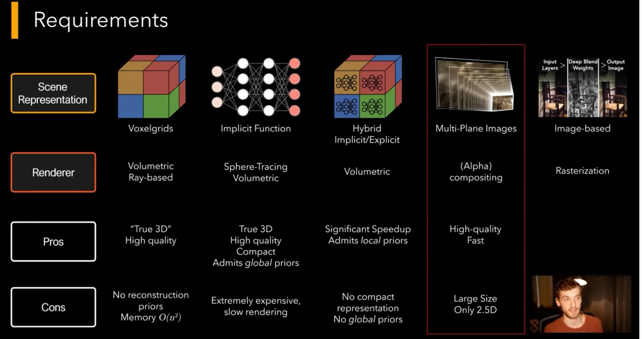
Multi Sphere Image, Multi-plane image (MPI), local layered representation format and DeepMPI representation (2.5 D), 2020
MSI: a Multi Sphere Image. LM: a Layered Mesh with individual layer textures. LM-TA: a Layered Mesh with a texture atlas.
Deep image or video generation approaches that enable explicit or implicit control of scene properties such as illumination, camera parameters, pose, geometry, appearance, and semantic structure. MPIs (rgba) have the ability to produce high-quality novel views of complex scenes in real time and the view consistency that arises from a 3D scene representation (in contrast to neural rendering approaches that decode a separate view for each desired viewpoint).
Our method takes in a set of images of a static scene, promotes each image to a local layered representation (MPI), and blends local light fields rendered from these MPIs to render novel views. As a rule of thumb, you should use images where the **maximum disparity between views is no more than about 64 pixels (watch the closest thing to the camera and don't let it move more than ~1/8 the horizontal field of view between images). Our datasets usually consist of 20-30 images captured handheld in a rough grid pattern. https://github.com/Fyusion/LLFF

 Its depth-wise resolution is limited by the number of discrete planes, and thus the MPIs cannot be converted to other 3D representations such as mesh, point cloud, etc. I
DeepMPI (2020) extends p
Synthesize plenoptic slices that can be interpolated to recover local regions of the full plenoptic function. Given a dense sampling of views, photorealistic novel views can be reconstructed by simple light field sample interpolation techniques. For novel view synthesis with sparser view sampling, the computer vision and graphics communities have made significant progress by predicting traditional geometry and appearance representations from observed images. The study of image-based rendering is motivated by a simple question: how do we use a finite set of images to reconstruct an infinite set of views.
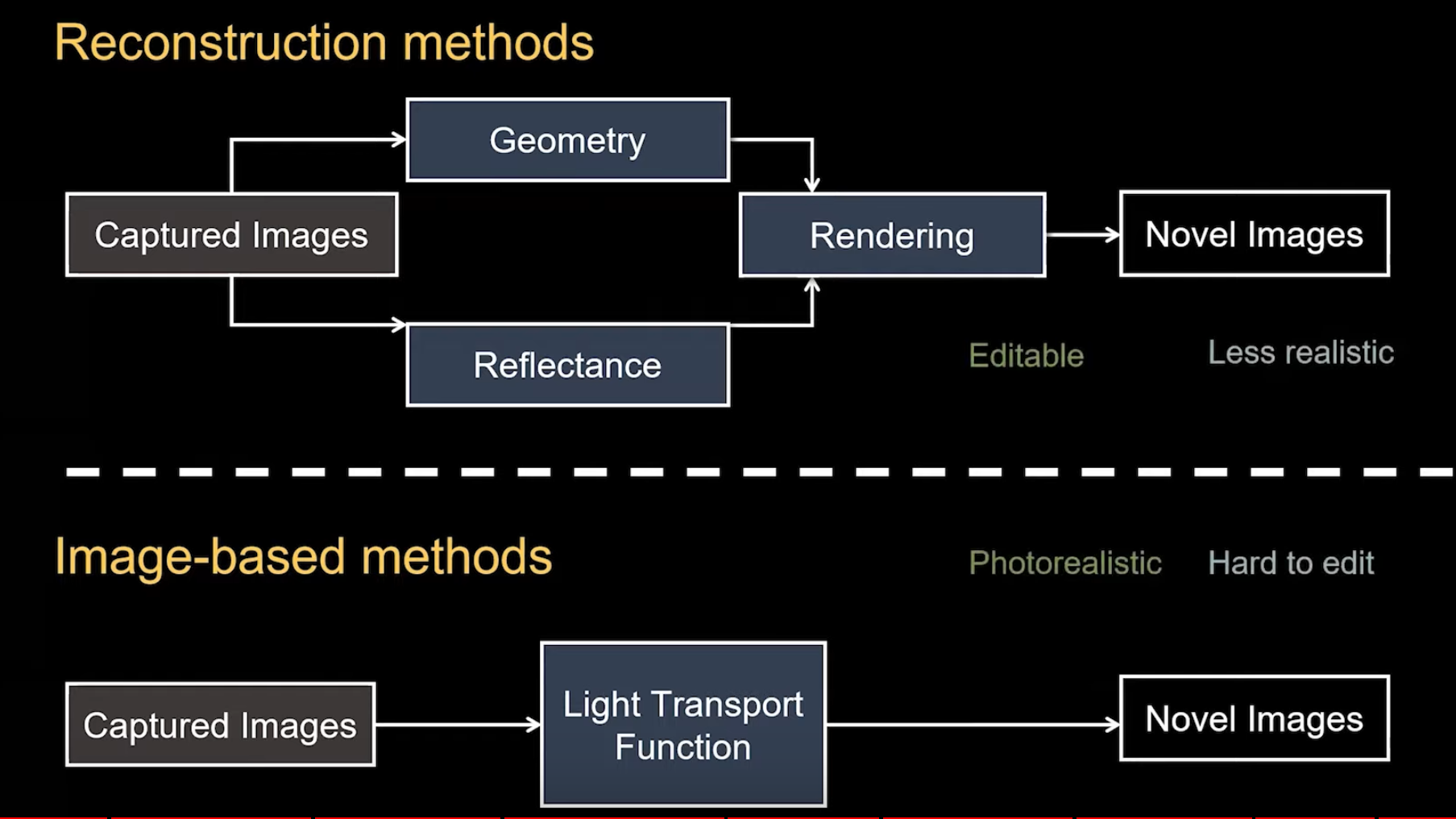
View synthesis can be approached by either explicit estimation of scene geometry and color, or using coarser estimates of geometry to guide interpolation between captured views. One approach aims to explicitly reconstruct the surface geometry and the appearance on the surface from the observed sparse views, other approaches adopt volume-based representations to directly to model the appearance of the entire space and use volumetric rendering techniques to generate images for 2D displays. The raw samples of a light field are saved as disks. resolution large amounts of data
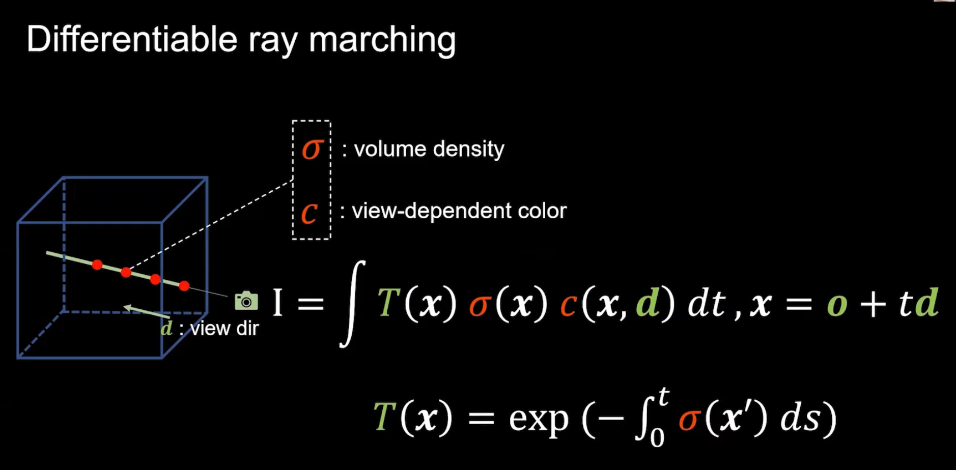
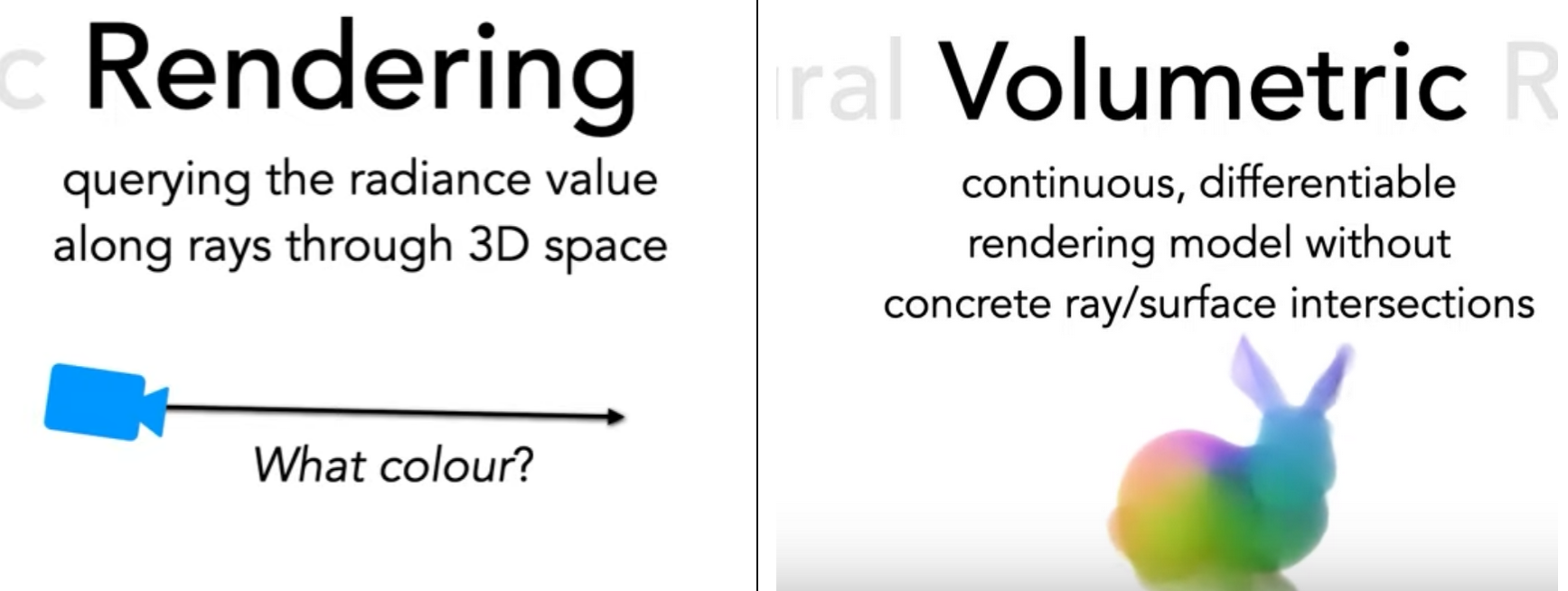
The Volume rendering technique known as ray marching. Ray marching is when you shoot out a ray from the observer (camera) through a 3D volume in space and ask a function: what is the color and opacity at this particular point in space? Neural rendering takes the next step by using a neural network to approximate this function.
Source: Advances in Neural Rendering, https://www.neuralrender.com/


Source: https://github.com/Arne-Petersen/Plenoptic-Simulation, A System for Acquiring, Processing, and Rendering Panoramic Light Field sStills for Virtual Reality
Source: Advances in Neural Rendering, https://www.neuralrender.com/
Light field rendering pushes the latter strategy to an extreme by using dense structured sampling of the lightfield to make re-construction guarantees independent of specific scene geometry. Most image based rendering algorithms are designed to model static appearance, DeepMPI (Deep Multiplane Images), which further captures viewing condition dependent appearance.
The key concept behind neural rendering approaches is that they are differentiable. A differentiable function is one whose derivative exists at each point in the domain. This is important because machine learning is basically the chain rule with extra steps: a differentiable rendering function can be learned with data, one gradient descent step at a time. Learning a rendering function statistically through data is fundamentally different from the classic rendering methods we described above, which calculate and extrapolate from the known laws of physics.
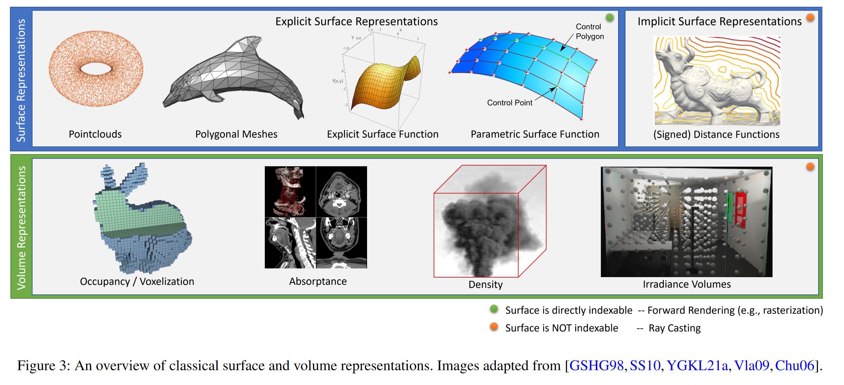
They can be classified into explicit and implicit representations. Explicit methods describe scenes as a collection of geometric primitives, such as triangles, point-like primitives, or higher-order parametric surfaces.
Source: Advances in Neural Rendering, https://www.neuralrender.com/
One popular class of approaches uses mesh-based representations of scenes with either use or view-dependent appearance. Differentiable rasterizers or pathtracers can directly optimize mesh representations to reproduce a set of input images using gradient descent. However, gradient-based mesh optimization based on image reprojection is often dicult, likely because of local minima or poor conditioning of the loss landscape. Furthermore, this strategy requires a template mesh with xed topology to be provided as an initialization before optimization [22], which is typically unavailable for unconstrained real-world scenes.
Inverse rendering aims to estimate physical attributes of a scene, e.g., reflectance, geometry, and lighting from image(s). Also called Differentiable Rendering it promises to close the loop between computer vision and graphics.
In this problem, a neural network learns to render a scene from an arbitrary viewpoint. Both of these works use a volume rendering technique known as ray marching. Ray marching is when you shoot out a ray from the observer (camera) through a 3D volume in space and ask a function: what is the color and opacity at this particular point in space? Neural rendering takes the next step by using a neural network to approximate this function.
Source: Advances in Neural Rendering, https://www.neuralrender.com/
Neural Radiance Fields (NeRF) rendering: Representing Scenes as Neural Radiance Fields, published 2020 Mildenhall
- https://www.youtube.com/watch?v=nCpGStnayHk Two Minute Papers explonation 2) Nerf (radiance fields) basics and encodings
Source: Advances in Neural Rendering, https://www.neuralrender.com/
For more about Nerfs go to next chapter https://github.com/3a1b2c3/seeingSpace/wiki/2)-Nerf-(radiance-fields)-basics,-frameworks-and-real-world-uses
-
Faster Training
-
Faster Inference and Rendering (see 6) Nerf rendering, compositing and web viewing)
-
Generalization, learning classes of objects
-
View Synthesis for Dynamic Scenes/ Video (see 5) Generative and dynamic Nerfs: Text to nerf
-
- Deformable/Animation
-
Compositionality (see 6) Nerf rendering, compositing and web viewing)
-
- Labelling and Depth Estimation (see 4) Nerf for relighting, mesh extraction, scene segmentation)
-
- Editing / Editable NeRFs (see 6) Nerf rendering, compositing and web viewing)


Source: https://medium.com/@hurmh92/autonomous-driving-slam-and-3d-mapping-robot-e3cca3c52e95
Over the past year (2020), we’ve learned how to make the rendering process differentiable, and turn it into a deep learning module. This sparks the imagination, because the deep learning motto is: “If it’s differentiable, we can learn through it”. If we know how to differentially go from 3D to 2D, it means we can use deep learning and backpropagation to go back from 2D to 3D as well.
With neural rendering we no longer need to physically model the scene and simulate the light transport, as this knowledge is now stored implicitly inside the weights of a neural network. The compute required to render an image is also no longer tied to the complexity of the scene (the number of objects, lights, and materials), but rather the size of the neural network.
Neural rendering has already enabled applications that were previously intractable, such as rendering of digital avatars without any manual modeling. Neural rendering could have a profound impact in making complex photo and video editing tasks accessible to a much broader audience.
This is no longer a neural network that is predicting physics. This is physics (or optics) plugged on top of a neural network inside a PyTorch engine. We have now a differentiable simulation of the real world (harnessing the power of computer graphics) on top of a neural representation of it.
https://towardsdatascience.com/three-grand-challenges-in-machine-learning-771e1440eafc Vincent Vanhoucke, Distinguished Scientist at Google This is why I call the grand challenge for perception the Inverse Video Game problem: predict not only a static scene but its functional semantics and possible futures. You should be able to take a video, run it through your computer vision model, and get a representation of a scene you can not only parse, but can roll forward in time to generate plausible future behaviors, from any viewpoint, like a video game engine would. It would respect the physics (a ball shot at a goal would follow its normal trajectory), semantics (a table would be movable, a door could be opened), and agents in the scene (people, cars would have reasonable NPC behaviors).
A lot of computer vision and graphics algorithms can be defined in a closed form solution, which therefore allows for optimizations.
Neural computing is very computationally expensive in part because (by design) it can’t be reduced to a closed form solution in the same way. Many of such closed-form contain infinite integral that are impossible to solve. We then use approximations (like Monte Carlo Markov Chain) but they take a long time to converge. It is really worth it to use a neural network to at list prototype and find the right settings before computing the final version.
Join Nerf discord at https://discord.gg/bRCMhXBg or the Nerfstudio discord at https://discord.gg/B2wb62hA and build the future with us